Table of Contents
- 1. Introduction of the author
- 2. Dataset introduction
-
- 2.1 Cifar-10 Dataset Introduction:
- 3. ResNet network introduction
-
- 3.1Residual Network residual network
- 3.2 ResNet18 network structure
- 4. Code reproduction and experimental results
-
- 4.1 Training code
- 4.2 Test code
- 4.3 Experimental results
1. Introduction of the author
An Yaohui, male, 22nd graduate student, School of Electronic Information, Xi’an Polytechnic University
Research direction: small sample image classification algorithm
E-mail: [email protected]
Zhang Siyi, female, School of Electronic Information, Xi’an Polytechnic University, 2022 graduate student, Zhang Hongwei Artificial Intelligence Research Group
Research direction: machine vision and artificial intelligence
Email: [email protected]
2. Dataset introduction
2.1 Cifar-10 Dataset Introduction:
The CIFAR-10 dataset consists of 60,000 images, each of which is a color image of size 32~32, and each category has 6,000 images. There are 50,000 training images and 10,000 testing images (10 classes in total, as shown).
The dataset is divided into five training batches and one testing batch, each with 10000 images. The test batch contains 1000 randomly selected images from each class. The training batches contain the remaining images in random order, but some training batches may contain more images from one class than another. Between them, the training batches contain exactly 5000 images from each class.

3. ResNet network introduction
3.1Residual Network residual network
The full name of ResNet is Residual Network residual network. Kaiming He’s “Deep Residual Learning for Image Recognition” won the best paper of CVPR. The deep residual network he proposed can be said to have washed away the major competitions in the image field in 2015, and won multiple championships with absolute advantages. Moreover, on the premise of ensuring the accuracy of the network, it increased the depth of the network to 152 layers, and later further increased the depth to 1000. The beginning of the paper first explained the benefits of deep networks: the feature level becomes higher with the deepening of the network, and the expressive ability of the network will also be greatly improved. Therefore, a question is raised in the paper: Can a better network be obtained by superimposing the number of network layers? The author found through experiments that the effect of a deep network that simply stacks the network is not as good as a shallower network with an appropriate number of layers. Therefore, He Yuming and others added a shortcut to the ordinary plain network to form a residual block. At this point, the fitting target becomes F(x), and F(x) is the residual:

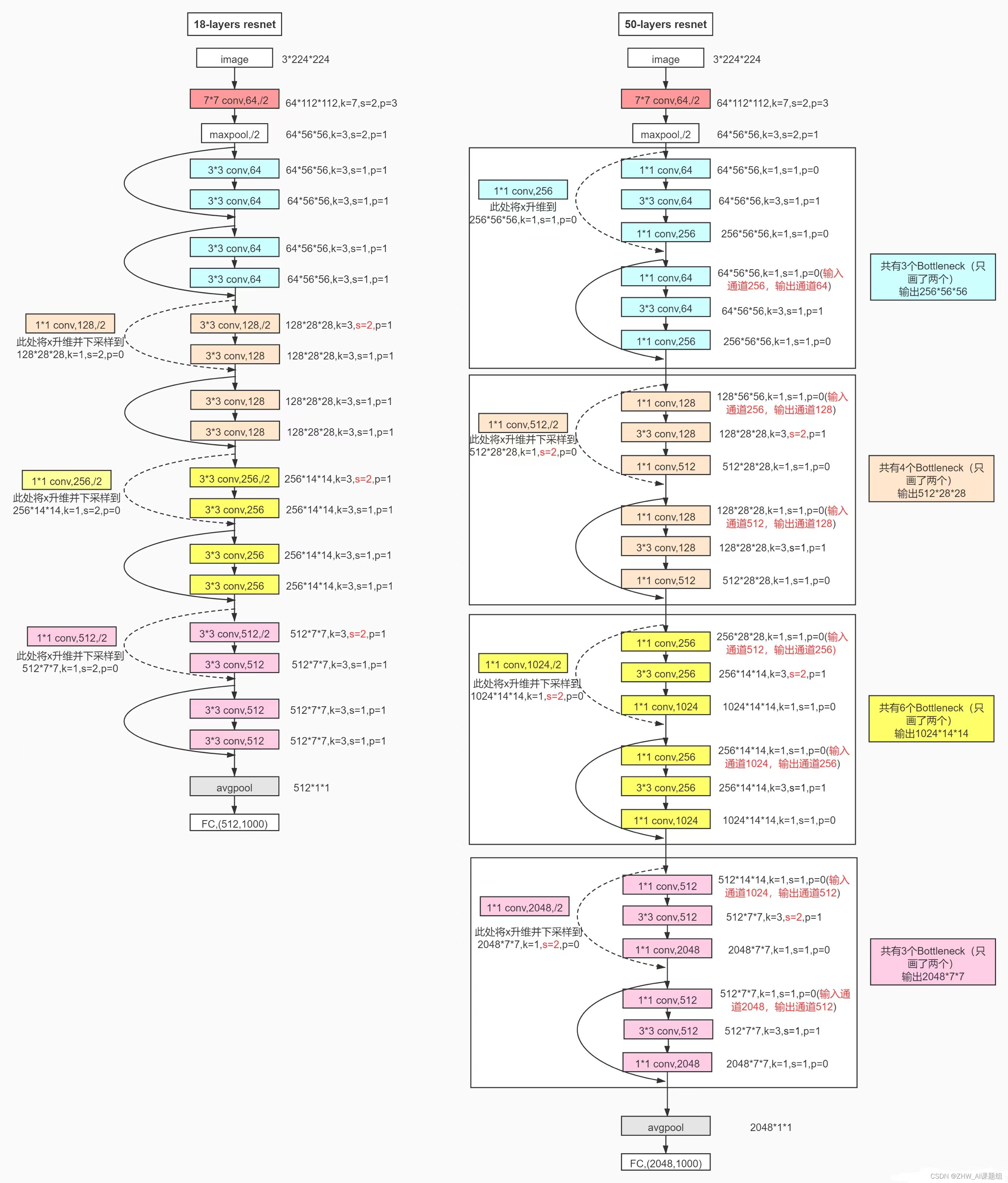
3.2 ResNet18 network structure
Here are more detailed ResNet18 network specific parameters and execution flow chart:
4. Code reproduction and experimental results
4.1 Training code
import torch
import numpy as np
from tqdm import tqdm
import torch.nn as nn
import torch.optim as optim
from utils.readData import read_dataset
from utils.ResNet import ResNet18

# set device
device = 'cuda' if torch.cuda.is_available() else 'cpu' # enable gpu
# read data
batch_size = 128
train_loader, valid_loader, test_loader = read_dataset(batch_size=batch_size,
                                                     pic_path='D:\AnYaohui\Cifar10\data')
# Load the model (use the preprocessed model, modify the last layer, fix the previous weights)
n_class = 10
model = ResNet18()
"""
The 7x7 downsampling convolution and pooling operations of the ResNet18 network tend to lose part of the information,
So in the experiment we removed the 7x7 downsampling layer and the maximum pooling layer and replaced it with a 3x3 downsampling convolution,
Reduce the stride and padding size of this convolutional layer at the same time
"""
model.conv1 = nn.Conv2d(in_channels=3, out_channels=64, kernel_size=3, stride=1, padding=1,
                        bias=False)
model.fc = torch.nn.Linear(512, n_class) # Change the last fully connected layer
model = model.to(device)
# Use the cross entropy loss function
criterion = nn.CrossEntropyLoss().to(device)

# start training
n_epochs = 250
valid_loss_min = np.Inf # track change in validation loss means + ∞, there is no exact value, and the type is floating point
accuracy = []
lr = 0.1
counter = 0
for epoch in tqdm(range(1, n_epochs + 1)):

    # keep track of training and validation loss
    train_loss = 0.0
    valid_loss = 0.0
    total_sample = 0
    right_sample = 0

    # Dynamically adjust the learning rate
    if counter/10 ==1:
        counter = 0
        lr = lr*0.5
    optimizer = optimize.SGD(model.parameters(), lr=lr, momentum=0.9, weight_decay=5e-4)
    ####################
    # Model for the training set #
    ####################
    model.train() #The role is to enable batch normalization and drop out
    for data, target in train_loader:
        data = data.to(device)
        target = target.to(device)
        # clear the gradients of all optimized variables (clear the gradient)
        optimizer. zero_grad()
        # forward pass: compute predicted outputs by passing inputs to the model
        # (forward pass: calculate the predicted output by passing the input to the model)
        output = model(data).to(device) # (equivalent to output = model.forward(data).to(device) )
        # calculate the batch loss (calculate the loss value)
        loss = criterion(output, target)
        # backward pass: compute gradient of the loss with respect to model parameters
        # (backward pass: calculate the gradient of the loss with respect to the model parameters)
        loss. backward()
        # perform a single optimization step (parameter update)
        # Execute a single optimization step (parameter update)
        optimizer. step()
        # update training loss (update loss)
        train_loss + = loss.item()*data.size(0)

    ########################
    # Validation set model#
    ########################

    model.eval() # Validate the model
    for data, target in valid_loader:
        data = data.to(device)
        target = target.to(device)
        # forward pass: compute predicted outputs by passing inputs to the model
        output = model(data).to(device)
        # calculate the batch loss
        loss = criterion(output, target)
        # update average validation loss
        valid_loss + = loss.item()*data.size(0)
        # convert output probabilities to predicted class (convert output probability to predicted class)
        _, pred = torch.max(output, 1)
        # compare predictions to true label (compare predictions to true labels)
        correct_tensor = pred.eq(target.data.view_as(pred))
        # correct = np. squeeze(correct_tensor. to(device). numpy())
        total_sample += batch_size
        for i in correct_tensor:
            if i:
                right_sample += 1
    print("Accuracy:",100*right_sample/total_sample,"%")
    accuracy.append(right_sample/total_sample)

    # Compute average loss
    train_loss = train_loss/len(train_loader.sampler)
    valid_loss = valid_loss/len(valid_loader.sampler)

    # Display the loss function of the training set and validation set
    print('Epoch: {} \tTraining Loss: {:.6f} \tValidation Loss: {:.6f}'.format(
        epoch, train_loss, valid_loss))

    # If the validation set loss function decreases, save the model.
    if valid_loss <= valid_loss_min:
        print('Validation loss decreased ({:.6f} --> {:.6f}).Saving model ...'.format(valid_loss_min,valid_loss))
        torch.save(model.state_dict(), 'checkpoint/resnet18_cifar10.pt')
        valid_loss_min = valid_loss
        counter = 0
    else:
        counter + = 1
4.2 Test code
import torch
import torch.nn as nn
from utils.readData import read_dataset
from utils.ResNet import ResNet18
# set device
device = 'cuda' if torch.cuda.is_available() else 'cpu'
n_class = 10
batch_size = 100
train_loader, valid_loader, test_loader = read_dataset(batch_size=batch_size, pic_path='dataset')
model = ResNet18() # Get the pre-trained model
model.conv1 = nn.Conv2d(in_channels=3, out_channels=64, kernel_size=3, stride=1, padding=1, bias=False)
model.fc = torch.nn.Linear(512, n_class) # modify the last fully connected layer
# load weights
model.load_state_dict(torch.load('checkpoint/resnet18_cifar10.pt'))
model = model.to(device)

total_sample = 0
right_sample = 0
model.eval() # Validate the model
for data, target in test_loader:
    data = data.to(device)
    target = target.to(device)
    # forward pass: compute predicted outputs by passing inputs to the model
    output = model(data).to(device)
    # convert output probabilities to predicted class (convert output probability to predicted class)
    _, pred = torch.max(output, 1)
    # compare predictions to true label (compare predictions to true labels)
    correct_tensor = pred.eq(target.data.view_as(pred))
    # correct = np. squeeze(correct_tensor. to(device). numpy())
    total_sample += batch_size
    for i in correct_tensor:
        if i:
            right_sample += 1
print("Accuracy:",100*right_sample/total_sample,"%")
4.3 Experimental results

