Table of Contents
1. Preview of algorithm operation renderings
2.Algorithm running software version
3. Some core programs
4. Overview of algorithm theory
5. Algorithm complete program engineering
1. Preview of algorithm operation renderings
2. Algorithm running software version
matlab2022a
3. Part of the core program
 Prn = NavData(PRNS_SEL,1);%Identify PRN in navigation data

        iode = NavData(PRNS_SEL,11);% enterprise date serial number

        Crs = NavData(PRNS_SEL,12);% orbit radius sinusoidal harmonic correction amplitude

        delta_n = NavData(PRNS_SEL,13);% average motion difference from calculated value

        M_zero = NavData(PRNS_SEL,14);% average anomaly at reference time

        Cuc = NavData(PRNS_SEL,15);% amplitude of the cosine harmonic correction term of the latitude variable

        es = NavData(PRNS_SEL,16);% eccentricity

        Cus = NavData(PRNS_SEL,17);% amplitude of the sine harmonic correction term of the latitude argument

        sqrt_a = NavData(PRNS_SEL,18);% square root of semi-major axis

        toe = NavData(PRNS_SEL,19);% ephemeris reappearance time (second time in GPS week)

        Cic = NavData(PRNS_SEL,20);% amplitude of the tilt cosine harmonic correction term

        OMEGA_zero = NavData(PRNS_SEL,21);% reference time right ascension

        Cis = NavData(PRNS_SEL,22);% amplitude of the sinusoidal harmonic correction term of the tilt angle

        i_zero = NavData(PRNS_SEL,23);% inclination angle of reference time

        Crc = NavData(PRNS_SEL,24);% orbit radius cosine harmonic correction amplitude

        omega = NavData(PRNS_SEL,25);%Perigee argument

        OMEGA_dot = NavData(PRNS_SEL,26);% right ascension angle change rate

        i_dot = NavData(PRNS_SEL,27);% slope change rate
       %Calculate true exception

       % corrected mean motion
        n_initial = sqrt(Gravitational_constant)/(sqrt_a*sqrt_a*sqrt_a);
        n = n_initial + delta_n;

       %Calculate time since reference epoch
        t_k = func_tk_limits(t,toe);

       %T_Kaverage anomaly
        M_k = M_zero + n * t_k + 2*pi;
        E_k = M_k;
        E_k1= M_k - es*sin(E_k);

        Iterative solution of %E_K
        while (abs(E_k - E_k1) > 1e-9)
            E_k1 = E_k;
            E_k = M_k + es * sin(E_k1);
        end;

        %TRUE ANOMALY
        v_k = 2*atan(sqrt((1 + es)/(1-es))*tan(E_k/2));
        %%latitude theory

        %The independent variable of uncorrected latitude
        phi_k = v_k + omega;

        %Correction
        C_u = Cus*sin(2*phi_k) + Cuc*cos(2*phi_k);
        C_r = Crs*sin(2*phi_k) + Crc*cos(2*phi_k);
        C_i = Cis*sin(2*phi_k) + Cic*cos(2*phi_k);
01_075m
4. Overview of Algorithm Theory
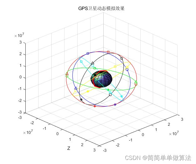
Simulating the orbital operation of 24 GPS satellites is a complex task that involves orbit calculation and drawing of multiple satellites. Below is a rough step-by-step and sample code for simulating and plotting the orbits of these satellites in MATLAB. The orbital parameters of actual GPS satellites are very complex, and the relative motion between satellites also needs to be considered. The sample code below is a simplified version to demonstrate the basic concepts. To simulate the orbital effects of 24 GPS satellites through MATLAB, you can follow the following steps:
Obtain satellite orbit parameters: The orbit parameters of GPS satellites can be obtained from relevant literature or data sources. These parameters include each satellite’s semi-major axis, eccentricity, orbital inclination, ascending node right ascension, etc.
Calculate the satellite’s orbit: Using the obtained orbital parameters, the position and velocity of each satellite at each point in time can be calculated through Kepler’s equations of motion.
Select a simulation time frame: Select an appropriate time frame to observe the motion of the satellite on the Earth.
Generate time series: To generate a series of time points, you can use the time function in MATLAB, such as linspace, to generate equally spaced time points.
Calculate satellite positions: For each time point, using the calculated orbital parameters and time, calculate the position and velocity of each satellite.
Draw satellite orbits: Use MATLAB’s drawing functions, such as plot3, to draw the orbit of each satellite in three-dimensional space. You can plot the satellite’s position on the Earth’s sphere, or you can plot its trajectory in a three-dimensional Cartesian coordinate system.
By using GPS satellite ephemeris (Almanac data) information, the orbits of 24 GPS satellites are calculated and simulated. Each satellite is numbered with PRN1-24, assuming that the GPS satellite orbit is circular.
Simulate the orbit of your own satellite. This satellite is a sun-synchronous orbit satellite 350Km above the ground. This orbit is elliptical, using an orbital inclination of 98 degrees
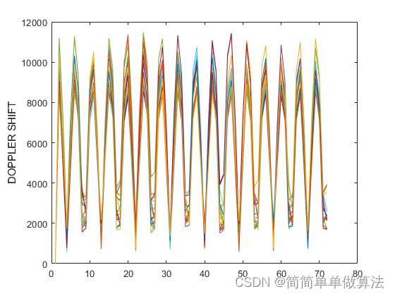
Calculate the Doppler shift of your own satellite and each GPS satellite.
Note: The GPS satellite used here is the sending source, and your own satellite is the receiving source. Assuming the transmission frequency is 1575.42 MHz
The orbital period of the GPS satellite is almost 24 hours, and the period of its own satellite in the sun-synchronous orbit is about 1.5 hours. This means that the sun-synchronous orbit has been around for several weeks, and the GPS satellite has only been around once. So when calculating the Doppler frequency shift, you only need to calculate the Doppler frequency shift within one GPS cycle. That is to say, if the Doppler frequency shift is calculated for more than 24 hours, the Doppler frequency shift will be repeated. All I need is the Doppler shift within the 24 hour GPS orbit period.
Here, first introduce the meaning of ephemeris files:
Prn
Satellite number
iode
The validity period of the current reference epoch given in the message
Crs
The correction term of the orbital radius and angular distance given in the message-sinusoidal amplitude
delta_n
Horizontal angle correction value given in the message
M_zero
Reference time mean approach angle given in the message
Cuc
The correction term of the right ascension of the ascending node given in the message-cosine amplitude
e1
The eccentricity of the orbital ellipse given in the message
Cus
The correction term of the right ascension of the ascending node given in the message-sine amplitude
sqrt_a
The square root of the semi-major axis of the satellite orbit ellipse given in the message
toe
Reference time given in the message
Cic
The correction term for the inclination angle distance given in the message-cosine amplitude
OMEGA_zero
The right ascension of the ascending node at the reference time given in the message
Cis
The correction term for the inclination angle distance given in the message-sinusoidal amplitude
i_zero
The reference time orbital inclination given in the message
Crc
The correction term of the orbital radius and angular distance given in the message-cosine amplitude
omega
The orbital perigee distance given in the message
OMEGA_dot
The rate of change of the right ascension of the ascending node given in the message
i_dot
The rate of change of orbital inclination given in the message
What needs to be paid attention to here is that since the height of GPS from the ground is generally 20,000km, and the geostationary satellite here is only 350km, the effect will not seem obvious, so here we set the parameters here to be larger, so that the effect looks slightly more obvious. point. Then when you write a paper, if you use the data, just change it back to 350. In addition, its cycle is 1.5 hours, so when in the house, the speed is too fast and it is not easy to observe. The setting here is slightly larger, and the use cycle is 6 hours.
5. Algorithm complete program engineering
OOOOO
OOO
O