Introduction
Perlin noise is designed to describe random effects in nature. It creates textures that can be applied directly to a vertex shader, rather than generating a texture map and then attaching the map to a three-dimensional object using traditional texture mapping techniques.
This is equivalent to the fact that the texture will not need to adapt to the surface. We only need to provide the (x, y, z) coordinates of each vertex, pass in the Perlin noise function Noise(), calculate a random number, and then compare it with the original color Operation to get new colors, just like drawing textures directly on the surface of the object. This means that our code that applies Perlin noise is best to use a shader and directly pass the color operation to the vertex shader.
Then, the key to the problem is what this Noise() should be like. Perlin believes that the noise function should satisfy the following properties:
1. Rotation statistical invariance. (It has the same statistical properties no matter how we rotate its domain)
2. There is a certain limit to the frequency bandpass. (It has no obvious big or small characteristics, but is within a certain range)
3. Translational statistical invariance. (It has the same statistical properties no matter how we translate its domain)
This means that we can create the random properties of the desired surface at different visual scales.

1. Preprocessing: Consider the set of all points in x, y, z space (coordinates are integers), we call this set an integer grid. Now we attach a pseudo-random gradient value on (x, y, z) to each point of the integer grid, which is a vector, and process it into a unit vector.
The calculation method given by perlin is as follows:
For each vertex, a vector is first randomly generated (for example, calling rand() in the C library), and then the subscript is fixedly mapped to another subscript, and the vertex vector corresponding to the other subscript is taken. If it is two-dimensional or three-dimensional, this process will be repeated twice. The specific process can be seen in the subsequent code.
2. If (x, y, z) is on the integer grid, then the noise here is d.
3. If (x, y, z) is not on the integer grid, we calculate the smooth interpolation coefficient.
The specific method is as follows. Taking two dimensions as an example, we need to find four integer points around this point, and then we get four values. The abscissa is bx0 ~ bx1, and the ordinate is by0 ~ by1. The distance from the point to bx0 on the x-axis is rx0, and the distance to by0 on the y-axis is ry0.
Perlin gives a smoothing curve to make linear interpolation coherent.
Evolution curve function that makes the first derivative continuous (original version): s_curve(t) ( t * t * (3. – 2. * t) )
Evolution curve function that makes the second derivative continuous (updated version): s_curve(t) ( t * t * t * (6 * t * t – 15 * t + 10) )
Then rx0 and ry0 are passed into the relaxation curve respectively to obtain new values sx and sy.
Next, do a bilinear interpolation. sx and sy are the coefficients of the linear interpolation in the first step, but after calculating the coefficients, we also need the starting point and end point of the interpolation. Their calculation method is as follows:
(1) Find the dot product of (rx0, ry0) and the gradient b00 of the upper left corner point to get the starting point u. Find the dot product of (rx0 + 1, ry0) and the gradient b10 of the upper right corner point to get the end point v. Let uv be At both ends, sx is the interpolation coefficient, and linear interpolation is performed to obtain a
(2) Find the dot product of (rx0, ry0 + 1) and the gradient b01 of the lower left corner point to get the starting point u. Find the dot product of (rx0 + 1, ry0 + 1) and the gradient b11 of the lower right corner point to get the end point v. , with uv as both ends and sx as the interpolation coefficient, perform linear interpolation to obtain b
(3) Finally, linear interpolation is performed on a and b, and the interpolation coefficient is sy to obtain the final result.
In the above algorithm steps, it actually doesn’t matter whether the x-axis or the y-axis is interpolated first.
The final Perlin noise distribution is between -1 ~ 1, and we can map it to the color difference we need (such as 0 ~ 255 or 0 ~ 1) to get the corresponding color.
Application
After calculating the noise, we can do some simple applications, such as creating a simple random surface texture:
color = white * Noise(point)
The point in the above formula is the coordinate of the point.
The effect is as follows. This image has a narrow bandwidth, and its details are only distributed within a specific interval. That is, the frequency spectrum of the texture does not have some central peak frequencies. The code for generating these graphs will be given later. The difference between the two images is just different parameters, they are both generated by Perlin noise.


The code to generate the above basic Perlin noise texture will be given later. Some subsequent deformations are obtained based on the Noise() function. You can try to achieve these effects yourself according to some formulas given by perlin. Of course, you can also try to simulate some effects yourself.
Of course, we can do something else. For example, when we may want different ranges of values to be mapped to different colors:
color = Colorful(Noise(k*point)
By multiplying by a constant k, we can get textures at different scales. This description seems a bit obscure. We can take a look at the final effect:

You can see that this context is similar to the simplest Perlin noise map, except that we map the RGB of a specific interval to a color. (via Colorful function)
We call the function describing the respective change rates (gradients) of Noise() on x, y, and z as DNoise().
If we want to create a bump texture map, we can also add some noise perturbation to the original normal (normal) to create a bump effect. With DNoise(), this behavior becomes very convenient:
normal = normal + Dnoise(point)
The final rendering is as follows:

Let’s do something more interesting.
We can add a 1/f fluctuation and simulate this signal through the following formula (superimpose octave at different frequencies to get a more realistic effect):

The derivative of the above 1/f spectrum function is a monotonic spectrum function, so we can create similar normal perturbations in all octave at the same time. Its pseudo code is as follows:
f=1
while f < pixel_freq
normal + = Dnoise ( f * point )
f*=2
This algorithm stops after calculating to the pixel level. The above algorithms are independent on a pixel-by-pixel basis, which means that calculating the color of a pixel does not need to depend on other pixels, so we can calculate each pixel in parallel and greatly increase the running speed.

Marble texture
We noticed that marble has various levels. We can use sine waves to make a simple color filter:
function boring_marble(point)
x = point[1]
return marble_color(sin(x))
In the above formula, Point[1] is the first component (x) of point, and marble_color() is a spline function that can map a number to a color vector.
If you want to simulate more realistic marble, you can add a perturbation:
function marble(point)
x = point[1] + turbulence(point)
return marble_color(sin(x))

This disturbance turbluence() function can be obtained through Noise(). Its specific algorithm is as follows:
function turbulence(p)
t=0
scale=1
while( scale > pixelsize)
t + = abs(Noise(p/scale) * scale)
scale /= 2
return t
Water texture
Suppose we want to simulate the surface of a wave. For simplicity, we use normal perturbations instead of modifying the values of surface points.
We do this using spherical waves, and for each wave center we will perturb the surface normal by a function of the circle from the surface to the center.
normal + = wave (point – center)
function wave (v)
return direction(v) * cycloid (norm (v))
We can use the Doise() direction of a certain set of points to generate randomly distributed unit spheres to create multiple centers.
function makewaves(n)
for i in [ 1 .. n ]
center [i] = direction (Dnoise ( i * [100 0 0] ))
return center
For example, if we want to create a wave with 20 sources, we can call it like this:
if begin_frame
center = makewaves(20)
for c in center
normal + = wave (point – c)
The effect made with the parameter of 20:

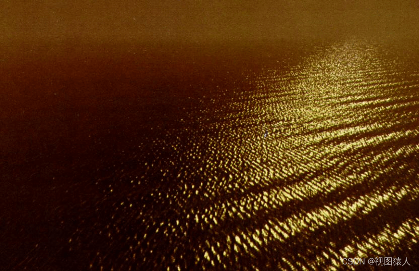
If you want to create a more realistic wave effect, you can add a 1/f disturbance. If we add a random frequency f to each center, then the last line of this program will be replaced by:
normal + = wave ((point – c) * f ) / f
Additionally, we need to make the waves move over time:
function moving_wave (v ,Dphase)
return direction(v) * cycloid (norm(v) – frame * Dphase)
Dphase is the speed of phase change. A parameter that can make the effect more realistic is f^(1/2).
The wave effect created:
The code of the basic Noise() function is given on perlin’s personal homepage. Only the two-dimensional part is intercepted below and the drawing part is added. For more detailed code, please refer to the following link. Click to open the link.
#include <stdlib.h>
#include "gl/glut.h"
#include <stdio.h>
#include <time.h>
#include <math.h>

#define B 0x100 //256
#defineBM 0xff //255

#define N 0x1000 //4096
#define NP 12 // 2^N
#define NM 0xfff

static int p[B + B + 2];
static float g2[B + B + 2][2];


int start = 1;

static void init(void);

//#define s_curve(t) ( t * t * (3. - 2. * t) )
#define s_curve(t) ( t * t * t * (t * (t * 6. - 15.) + 10.) )
#define lerp(t, a, b) ( a + t * (b - a) )
#define setup(i,b0,b1,r0,r1)\
t = vec[i] + N; \
b0 = ((int)t) & BM; \
b1 = (b0 + 1) & BM; \
r0 = t - (int)t; \
r1 = r0 - 1.;

float noise2(float vec[2])
{
int bx0, bx1, by0, by1, b00, b10, b01, b11;
float rx0, rx1, ry0, ry1, *q, sx, sy, a, b, u, v, t;
register int i, j;
if (start){
start = 0;
init();
    }
setup(0, bx0, bx1, rx0, rx1);
setup(1, by0, by1, ry0, ry1);
i = p[bx0];
j = p[bx1];

b00 = p[i + by0];
b10 = p[j + by0];
b01 = p[i + by1];
b11 = p[j + by1];

sx = s_curve(rx0);
sy = s_curve(ry0);

#define at2(rx,ry) ( rx * q[0] + ry * q[1] )
q = g2[b00]; u = at2(rx0, ry0);
q = g2[b10]; v = at2(rx1, ry0);
a = lerp(sx, u, v);

q = g2[b01]; u = at2(rx0, ry1);
q = g2[b11]; v = at2(rx1, ry1);
b = lerp(sx, u, v);

return lerp(sy, a, b);

}
static void normalize2(float v[2])
{
floats;
s = sqrt(v[0] * v[0] + v[1] * v[1]);
v[0] = v[0] / s;
v[1] = v[1] / s;
}

static void init(void)
{
int i, j, k;
for (i = 0; i < B; i + + ) {
p[i] = i;
for (j = 0; j < 2; j + + )
g2[i][j] = (float)((rand() % (B + B)) - B) / B;
}

while (--i) {
k = p[i];
p[i] = p[j = rand() % B];
p[j] = k;
}
for (i = 0; i < B + 2; i + + ){
p[B + i] = p[i];
for (j = 0; j < 2; j + + )
g2[B + 1][j] = g2[i][j];
}
}

void drawScene()
{
float d1 = -300.0, d2 = -300.0;
const float size = 0.1f;
for (int i = 0; i < 100; i + + ) {
d1 = -300;
for (int j = 0; j < 100; j + + ) {
float vec[2] = { d1,d2 };
float color = (noise2(vec) + 1)/4;
glColor3f(color,color,color);
glRectf(i*size, j*size, i*size + size, j*size + size);
d1 + = 0.1;
}
d2 + = 0.1;
}
}

void reshape(int width, int height)
{
if (height == 0)height = 1;
glViewport(0, 0, width, height);
glMatrixMode(GL_PROJECTION);//Set the matrix mode to projection
glLoadIdentity(); //Initialize the matrix to the identity matrix
glOrtho(0, 10,0,10, -100, 100); //Orthographic projection
glMatrixMode(GL_MODELVIEW); //Set matrix mode to model
}

void redraw()
{
glClear(GL_COLOR_BUFFER_BIT | GL_DEPTH_BUFFER_BIT);//Clear the color and depth cache
glMatrixMode(GL_MODELVIEW);
glLoadIdentity(); //Initialize the matrix to the identity matrix
drawScene();//Draw the scene
glutSwapBuffers();//Swap buffers
}

int main(int argc,char* argv[])
{
srand(time(nullptr));
glutInit(&argc, argv);//Initialization of glut
glutInitDisplayMode(GLUT_RGBA | GLUT_DEPTH | GLUT_DOUBLE);
glutInitWindowSize(400, 400);//Set the window size
int windowHandle = glutCreateWindow("Perlin Noise");//Set the window title
glutDisplayFunc(redraw); //Register drawing callback function
glutReshapeFunc(reshape); //Register the redraw callback function

glutMainLoop(); // glut event processing loop
}