Click “Xiaobai learns vision” above, and choose to add “Star” or “Stick“
Heavy dry goods, delivered as soon as possible
Particle Filter – Kidnapped vehicle project
Github: https://github.com/williamhyin/CarND-Kidnapped-Vehicle
Email: [email protected]
1. Definition of Particle Filter
A particle filter is an implementation of a Bayesian filter or a Markov localization filter. Particle filters are mainly used to solve localization problems based on the “principle of survival of the fittest”. Particle filters have the advantage of being easy to program and flexible.
Performance comparison of the three filters:

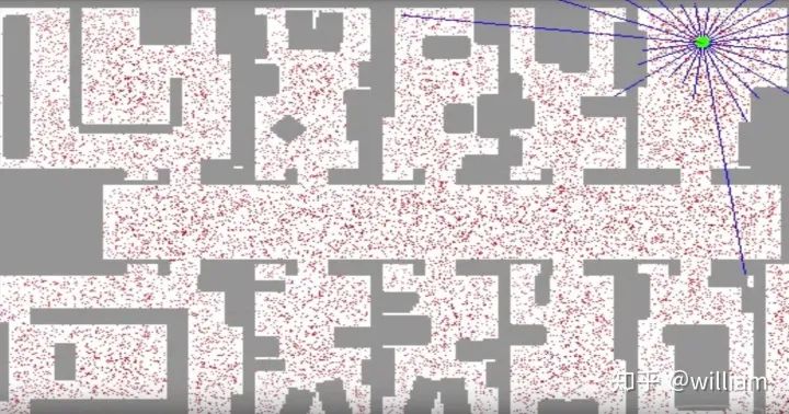
As you can see in the image above, the red dots are discrete guesses at where the robot might be. Each red point has an x-coordinate, y-coordinate, and direction. A particle filter is represented by a robotic posterior reliability representation consisting of a few thousand such guesses. At first, the particles are evenly distributed, but the fraction of the filter that keeps them alive is proportional to the agreement of the particles with the sensor’s measurement.
1. Weights:

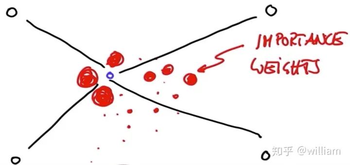
Particle filters typically carry a discrete number of particles. Each particle is a vector containing an x-coordinate, y-coordinate, and direction. Particle survival depends on their consistency with sensor measurements. Consistency is measured based on how well the actual and predicted measurements match, known as weights.

The weight means how close the actual measurement of the particle is to the predicted measurement. In a particle filter, the greater the particle weight, the higher the probability of survival. In other words, the survival probability of each particle is proportional to the weight.
2. Resampling
The resampling technique is used to randomly select N new particles from the old particles, and replace them proportionally according to the important weight. After resampling, particles with heavier weights may stick around and others may disappear. Particles gather in areas with relatively high posterior probabilities.
For resampling, the resampling round technique is employed.
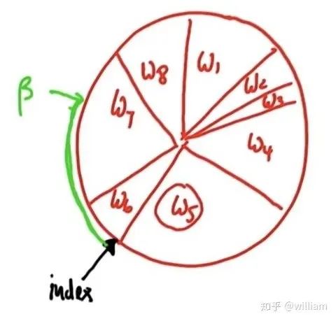

Principle: The probability of each particle being selected is proportional to the perimeter of the particle wheel. Particles with larger weights have more chances to be selected.
The initial index is 6, assuming random beta = 0 + random weight > w6, then index + 1, beta = beta-w6. At this time, beta < w7, particle No. 7 is selected and added to the warehouse. Then proceed to the next cycle, at this time beta and index still retain the value of the previous cycle, beta= beta + random weight > w7 + w8, so the index is incremented twice to reach index=1, at this time w1 > beta, w1 It is selected to be placed in the warehouse, and then the next round of circulation is carried out.
Code for resampling:
python p3 = [] index= int(random.random()*N) beta=0.0 mw=max(w) for i in range(N): beta + =random.random()*2.0*mw while beta>w[index]: beta-=w[index] index=(index + 1)%N p3.append(p[index]) p=p3
2. Particle Filters implementation
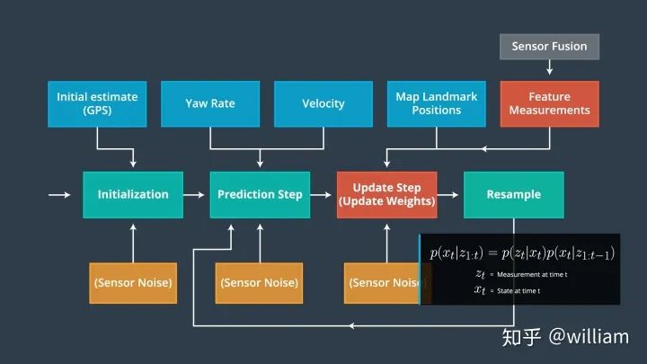
Particle filters have four main steps:
Initialization steps:
-
Initialization step: We estimate our position from the GPS input. Subsequent steps in the process will refine this estimate to localize our vehicle
-
Prediction step: In the prediction step, we add the control inputs (yaw velocity and velocity) of all particles
-
Particle weight update step: In the update step, we update the particle weights using measurements of map landmark positions and features
-
Resampling step: During resampling, we will resample m times (m is the range from 0 to length_of_particleArray) to draw particle i (i is the particle index) proportional to its weight. This step uses the resampling round technique.
-
The new particles represent Bayesian filtered posterior probabilities. We now have an accurate estimate of the vehicle’s position based on input proofs.
pseudocode:
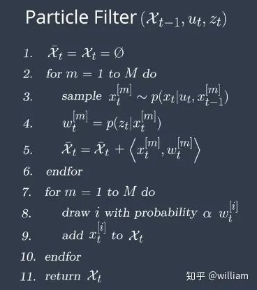
1. Initialization steps:
The first thing the particle filter does is initialize all the particles. In this step we have to decide how many particles to use. In general, we have to come up with a good number, because if it is not too small, it will be error-prone, and if it is too many, it will slow down the Bayesian filter. The traditional method of particle initialization is to divide the state space into a grid and place a particle in each cell, but this method can only be suitable for small state spaces, which is not suitable if the state space is the earth. It is therefore most practical to use GPS position input as an initial estimate of our particle distribution. It is worth noting that the measurement results of all sensors are bound to be accompanied by noise. In order to simulate the real uncontrollable noise situation, it should be considered to add Gaussian noise to the initial GPS position and heading of this project.
The final initialization step code of the project:
“`c ++ void ParticleFilter::init(double x, double y, double theta, double std[]) { /* * TODO: Set the number of particles. Initialize all particles to * first position (based on estimates of x, y, theta and their uncertainties * from GPS) and all weights to 1. * TODO: Add random Gaussian noise to each particle. * NOTE: Consult particle_filter.h for more information about this method * (and others in this file)./
if (is_initialized) {
       return;
   }
   num_particles = 100; // TODO: Set the number of particles
   double std_x = std[0];
   double std_y = std[1];
   double std_theta = std[2];

   // Normal distributions normal_distribution<double> dist_x(x, std_x);
   normal_distribution<double> dist_y(y, std_y);
   normal_distribution<double> dist_theta(theta, std_theta);

   // Generate particles with normal distribution with mean on GPS values. for (int i = 0; i < num_particles; + + i) {
       Particle pe;
       pe.id = i;
       pe.x = dist_x(gen);
       pe.y = dist_y(gen);
       pe.theta = dist_theta(gen);
       pe.weight = 1.0;
       particles.push_back(pe);

   }
   is_initialized = true;
2. Prediction steps:
Now that we have initialized the particles, it’s time to predict the position of the vehicle. Here, we will use the formula below to predict where the vehicle will be at the next time step, with yaw velocity and velocity based updates, while accounting for Gaussian sensor noise.

The project’s final prediction step code:
“`c++ void ParticleFilter::prediction(double delta_t, double std_pos[], double velocity, double yaw_rate) { /* * TODO: Add measurements to each particle and add random Gaussian noise. * NOTE: When adding noise you may find std::normal_distribution * and std::default_random_engine useful. * http://en.cppreference.com/w/cpp/numeric/random/normal_distribution * http://www.cplusplus.com/reference/ random/default_random_engine/ / //Normal distributions for sensor noise normal_distribution disX(0, std_pos[0]); normal_distribution disY(0, std_pos[1]); normal_distribution angle_theta(0, std_pos[2]);
for (int i = 0; i < num_particles; i ++ ) {
       if (fabs(yaw_rate) >= 0.00001) {
           particles[i].x + = (velocity / yaw_rate) * (sin(particles[i].theta + yaw_rate * delta_t) - sin(particles[i].theta));
           particles[i].y + = (velocity / yaw_rate) * (cos(particles[i].theta) - cos(particles[i].theta + yaw_rate * delta_t));
           particles[i].theta + = yaw_rate * delta_t;
       }
       else {
           particles[i].x + = velocity * delta_t * cos(particles[i].theta);
           particles[i].y + = velocity * delta_t * sin(particles[i].theta);
       }
       //Add noise
       particles[i].x + = disX(gen);
       particles[i].y + = disY(gen);
       particles[i].theta + = angle_theta(gen);

   }
} “`
3, Update steps:
Now that we have velocity and yaw rate measurement inputs into our filter, we must update the particle weights based on lidar and radar landmark readings.
The update step has three main steps:
-
Transformation
-
Association
-
Update Weights
-
Transformation
We first need to transform the car’s measurements from the local car coordinate system to the coordinate system on the map.
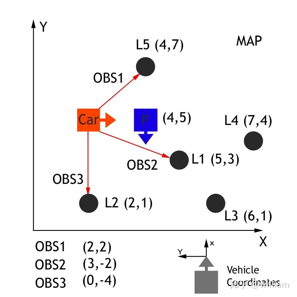
By passing vehicle observation coordinates (xc and yc), map particle coordinates (xp and yp), and our rotation angle (-90 degrees), observations in the vehicle coordinate system can be converted to map coordinates (xm and ym). This homogeneous transformation matrix, shown below, performs rotation and translation.
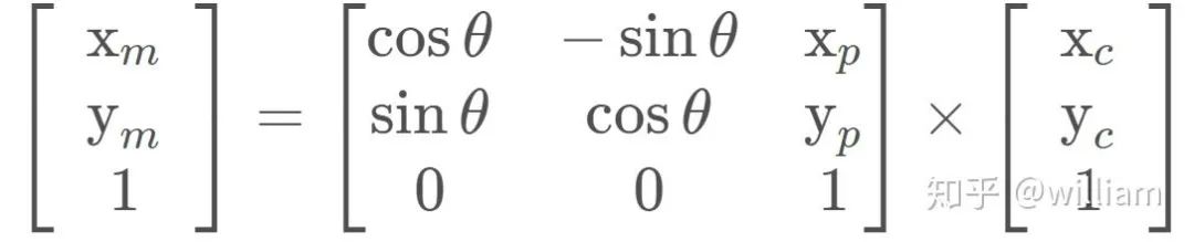
The result of matrix multiplication is:

code:c + + double x_part, y_part, x_obs, y_obs, theta; double x_map; x_map = x_part + (cos(theta) * x_obs) - (sin(theta) * y_obs); double y_map; y_map = y_part + ( sin(theta) * x_obs) + (cos(theta) * y_obs);
Remarks: The black box is a particle, we need to update its weight, (4,5) is its position in the map coordinates, its heading is (-90 degrees), because the sensor’s measurement of the road sign is based on the vehicle Its own coordinates, so we need to convert the observation data of the vehicle into map coordinates. For example, the real map coordinates of the L1 road sign are (5,3), the vehicle coordinates of OBS2 measured by the vehicle sensor are (2,2), and the map coordinates after homogeneous matrix transformation are (6,3), now we can Relate the measurements to the ground truth, matching landmarks in the real world, thereby updating the weights of the black boxed particles.
-
Contact (Association )
The linkage problem is the problem of matching landmark measurements to objects in the real world, such as map landmarks. Our ultimate goal is to find a weight parameter for each particle that represents how closely this particle matches the actual car in the same position.

Now that the observations have been transformed into the map’s coordinate space, the next step is to associate each transformed observation with a place identifier. In the map exercise above, we have a total of 5 landmarks, each identified as L1, L2, L3, L4, L5, each with a known map location. We need to associate each transition observation TOBS1, TOBS2, TOBS3 with one of these 5 identifiers. In order to do this, we must associate the closest landmarks with each transformed observation.TOBS1 = (6,3), TOBS2 = (2,2) and TOBS3 = (0,5). OBS1 matches L1, OBS2 Match L2, OBS3 matches L2 or L5 (same distance).
The following example explains the problem of data association.
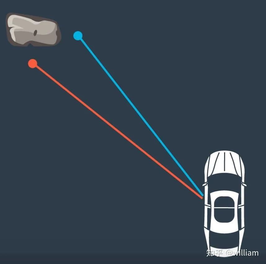
In this case we have two lidars measuring rocks. We need to find out which of these two measurements corresponds to the rock. If we estimate that any measurement is true, the position of the car will be different according to the measurement we choose. That is to say, depending on the choice of road signs, the final vehicle position will be different.
Since we have multiple measured landmarks, we can use the nearest neighbor technique to find the correct one.
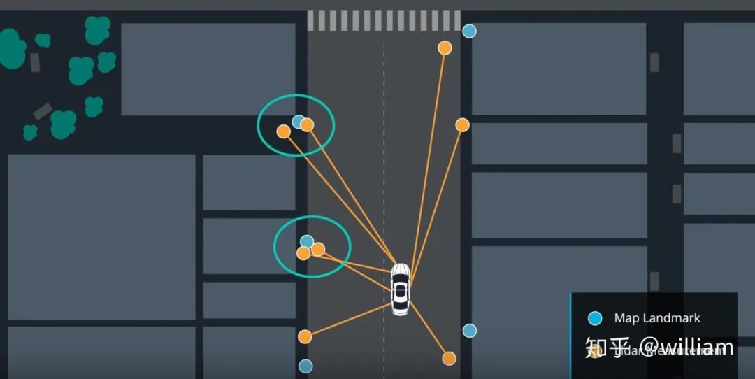
In this approach, we take the closest measurement as the correct one.
Advantages and disadvantages of the nearest neighbor method:

-
update weights
Now that we’ve done the measurement conversion and correlation, we have all the pieces we need to calculate the final weights of our particles. The final weight of the particle will be calculated as the product of each measured multivariate-Gaussian probability density.
A multivariate-Gaussian probability density has two dimensions, x and y. The mean of the multivariate Gaussian distribution is the relative landmark position of the measurement, and the standard deviation of the multivariate Gaussian distribution is described by our initial uncertainty in the range of x and y. The multivariate-Gaussian evaluation is based on the transformed measurement positions. The formula for the multivariate Gaussian distribution is as follows.

Remarks: x, y are the observed values in the map coordinate system, and μx, μy are the map coordinates of the nearest landmark. For example, for OBS2 (x,y) =(2,2), (μx, μy)= (2,1)
Error calculation formula:
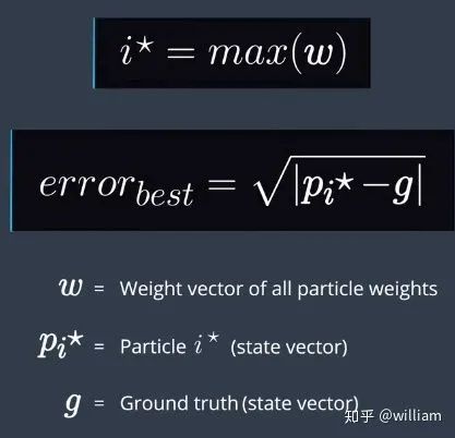

Where x, y, theta represent the best particle position, xmeas, ymeas, thetameas represent the real value
Item’s final weight update code:
void ParticleFilter::updateWeights(double sensor_range, double std_landmark[],
                                   const vector<LandmarkObs> & observations,
                                   const Map & map_landmarks) {
    /**
     * TODO: Update the weights of each particle using a mult-variate Gaussian
     * distribution. You can read more about this distribution here:
     * https://en.wikipedia.org/wiki/Multivariate_normal_distribution
     * NOTE: The observations are given in the VEHICLE'S coordinate system.
     * Your particles are located according to the MAP'S coordinate system.
     * You will need to transform between the two systems. Keep in mind that
     * this transformation requires both rotation AND translation (but no scaling).
     * The following is a good resource for the theory:
     * https://www.willamette.edu/~gorr/classes/GeneralGraphics/Transforms/transforms2d.htm
     * and the following is a good resource for the actual equation to implement
     * (look at equation 3.33) http://planning.cs.uiuc.edu/node99.html
     */
    double stdRange = std_landmark[0];
    double stdBearing = std_landmark[1];
    //Each particle for loop
    for (int i = 0; i < num_particles; i ++ ) {
        double x = particles[i].x;
        double y = particles[i].y;
        double theta = particles[i].theta;
// double sensor_range_2 = sensor_range * sensor_range;
        // Create a vector to hold the map landmark locations predicted to be within sensor range of the particle
        vector<LandmarkObs> validLandmarks;
        // Each map landmark for loop
        for (unsigned int j = 0; j < map_landmarks.landmark_list.size(); j ++ ) {
            float landmarkX = map_landmarks.landmark_list[j].x_f;
            float landmarkY = map_landmarks.landmark_list[j].y_f;
            int id = map_landmarks.landmark_list[j].id_i;
            double dX = x - landmarkX;
            double dY = y - landmarkY;
            /*if (dX * dX + dY * dY <= sensor_range_2) {
                inRangeLandmarks.push_back(LandmarkObs{ id,landmarkX,landmarkY });
            }*/
            // Only consider landmarks within sensor range of the particle (rather than using the "dist" method considering a circular region around the particle, this considers a rectangular region but is computationally faster)
            if (fabs(dX) <= sensor_range & amp; & amp; fabs(dY) <= sensor_range) {
                validLandmarks.push_back(LandmarkObs{id, landmarkX, landmarkY});
            }
        }
        // Create and populate a copy of the list of observations transformed from vehicle coordinates to map coordinates
        vector<LandmarkObs> transObs;
        for (int j = 0; j < observations. size(); j ++ ) {
            double tx = x + cos(theta) * observations[j].x - sin(theta) * observations[j].y;
            double ty = y + sin(theta) * observations[j].x + cos(theta) * observations[j].y;
            transObs.push_back(LandmarkObs{observations[j].id, tx, ty});
        }

        // Data association for the predictions and transformed observations on current particle
        dataAssociation(validLandmarks, transObs);
        particles[i].weight = 1.0;

        for (unsigned int j = 0; j < transObs. size(); j ++ ) {
            double observationX = transObs[j].x;
            double observationY = transObs[j].y;
            int landmarkId = transObs[j].id;

            double landmarkX, landmarkY;
            int k = 0;
            int nlandmarks = validLandmarks. size();
            bool found = false;
            // x,y coordinates of the prediction associated with the current observation
            while (!found & amp; & amp; k < nlandmarks) {
                if (validLandmarks[k].id == landmarkId) {
                    found = true;
                    landmarkX = validLandmarks[k].x;
                    landmarkY = validLandmarks[k].y;
                }
                k++;
            }
            // Weight for this observation with multivariate Gaussian
            double dX = observationX - landmarkX;
            double dY = observationY - landmarkY;
            double weight = (1 / (2 * M_PI * stdRange * stdBearing)) *
                            exp(-(dX * dX / (2 * stdRange * stdRange) + (dY * dY / (2 * stdBearing * stdBearing))));
            // Product of this obersvation weight with total observations weight
            if (weight == 0) {
                particles[i].weight = particles[i].weight * 0.00001;

            } else {
                particles[i].weight = particles[i].weight * weight;
            }
        }
    }
}
-
Resample step
The resampling technique is used to randomly sample new particles from old particles and replace them proportionally according to the importance weight. After resampling, particles with heavier weights may stick around and others may disappear. This is the final step of the particle filter.
Final resampling code for the project:
void ParticleFilter::resample() {
    /**
        * TODO: Resample particles with replacement with probability proportional
        * to their weight.
        * NOTE: You may find std::discrete_distribution helpful here.
        * http://en.cppreference.com/w/cpp/numeric/random/discrete_distribution
        */
    // Get weights and max weight.
    vector<double> weights;
    double maxWeight = numeric_limits<double>::min();
    for (int i = 0; i < num_particles; i ++ ) {
        weights.push_back(particles[i].weight);
        if (particles[i].weight > maxWeight) {
            maxWeight = particles[i].weight;
        }
    }
    uniform_real_distribution<float> dist_float(0.0, maxWeight);
    uniform_real_distribution<float> dist_int(0.0, num_particles - 1);
    int index = dist_int(gen);
    double beta = 0.0;
    vector<Particle> resampledParticles;
    for (int i = 0; i < num_particles; i ++ ) {
        beta += dist_float(gen) * 2.0;
        while (beta > weights[index]) {
            beta -= weights[index];
            index = (index + 1) % num_particles;
        }
        resampledParticles.push_back(particles[index]);
    }
    particles = resampledParticles;

}
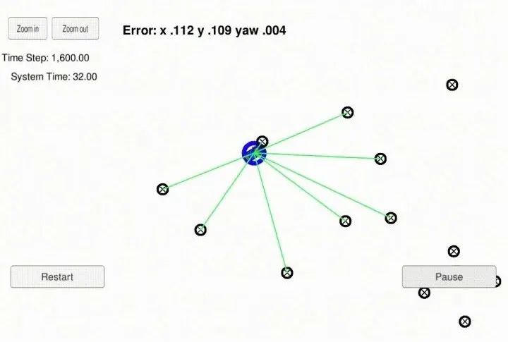
3. Project Demo
Good news!
Xiaobai learns visual knowledge planet
Open to the outside world

Download 1: OpenCV-Contrib extension module Chinese version tutorial

Reply in the backstage of the "Xiaobai Xue Vision" public account: Chinese tutorial of extension module, you can download the first Chinese version of OpenCV extension module tutorial on the whole network, covering extension module installation, SFM algorithm, stereo vision, target tracking, biological vision, super Resolution processing and more than 20 chapters.


Download 2: Python visual combat project 52 lectures
Reply in the background of the "Xiaobai Xue Vision" public account: Python visual combat project, you can download including image segmentation, mask detection, lane line detection, vehicle counting, adding eyeliner, license plate recognition, character recognition, emotion detection, text content extraction, Facial recognition and other 31 visual combat projects help fast school computer vision.


Download 3: OpenCV Practical Project 20 Lectures
Reply in the background of the "Xiaobai Xue Vision" public account: 20 lectures on OpenCV practical projects, you can download 20 practical projects based on OpenCV to achieve advanced OpenCV learning.


Exchange group

Welcome to join the reader group of the official account to communicate with peers. Currently, there are WeChat groups such as SLAM, 3D vision, sensors, automatic driving, computational photography, detection, segmentation, recognition, medical imaging, GAN, algorithm competitions (will be gradually subdivided in the future), Please scan the WeChat ID below to join the group, and remark: "nickname + school/company + research direction", for example: "Zhang San + Shanghai Jiaotong University + visual SLAM". Please make notes according to the format, otherwise it will not be approved. After the addition is successful, it will be invited to enter the relevant WeChat group according to the research direction. Please do not send advertisements in the group, otherwise you will be asked to leave the group, thank you for understanding~