?About the author: A Matlab simulation developer who loves scientific research. He cultivates his mind and improves his technology simultaneously.
For code acquisition, paper reproduction and scientific research simulation cooperation, please send a private message.
Personal homepage: Matlab Research Studio
Personal credo: Investigate things to gain knowledge.
For more Matlab complete code and simulation customization content, click
Intelligent optimization algorithm Neural network prediction Radar communication Wireless sensor Power system
Signal processing Image processing Path planning Cellular automaton Drone
Content introduction
GPS interference has always been a serious problem, affecting the reliability and accuracy of the global positioning system. Interference can come from a variety of sources, including radio frequency interference, electromagnetic radiation, and interference from other electronic devices. To solve this problem, researchers have been working hard to develop anti-interference algorithms and techniques.
In this article, we will introduce a Matlab-based GPS anti-interference link simulation algorithm process. This algorithm flow can help researchers simulate and evaluate different anti-jamming methods to improve the robustness and performance of GPS systems.
First, we need to prepare some necessary tools and data. This includes Matlab software, GPS signal models and interference models. Matlab is a very powerful mathematical modeling and simulation tool that can help us implement complex algorithms and models. The GPS signal model is a mathematical model that describes the GPS signal transmission process, including signal propagation, reception and demodulation. The interference model is a mathematical model that describes the interference signal, including the frequency, power, waveform and other characteristics of the interference signal.
Next, we need to write Matlab code to implement our algorithm flow. First, we need to generate the GPS signal and jamming signal. The GPS signal can be generated by the GPS signal model, and the interference signal can be generated by the interference model. Then, we need to superimpose the GPS signal and the interference signal to simulate the actual GPS signal reception process. Next, we need to write a demodulation algorithm to extract the navigation data from the GPS signal. This is achieved through the process of demodulating the GPS signal, including steps such as carrier frequency and chip synchronization, chip demodulation and navigation data decoding.
During the demodulation process, we need to consider the impact of interference on the GPS signal. Interfering signals may cause the signal-to-noise ratio to decrease, thereby affecting the accuracy and reliability of navigation data. In order to solve this problem, we can adopt some anti-interference methods, such as filtering, interference cancellation and adaptive signal processing technologies. These methods can help us resist interference and improve the performance of GPS systems.
During the simulation process, we can evaluate different anti-interference methods by changing the characteristics and parameters of the interference signal. By comparing the performance of different methods, we can choose the anti-interference method that best suits our application scenario. In addition, we can evaluate the impact of different GPS system configurations and parameters on anti-jamming performance to optimize system design and performance.
To sum up, the Matlab-based GPS anti-interference link simulation algorithm flow can help us simulate and evaluate different anti-interference methods to improve the robustness and performance of the GPS system. Through this process, we can better understand the working principle of the GPS system and the impact of interference on system performance. It is hoped that this algorithm process can help research and solve the problem of GPS interference and promote the further development of GPS technology.
Part of the code
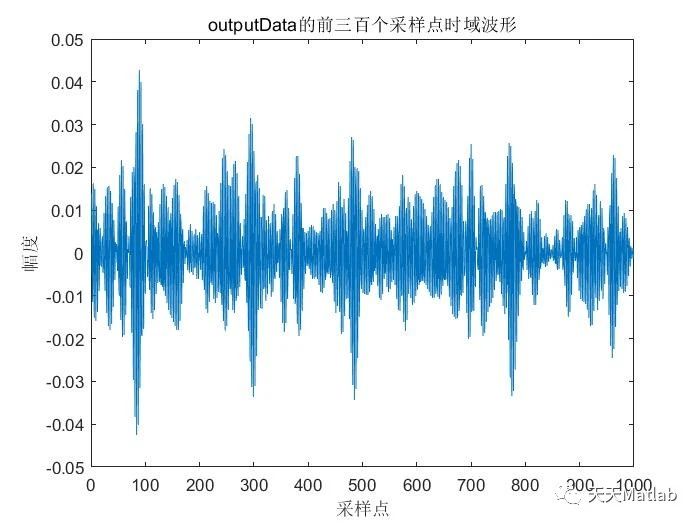
function probeData(varargin)</code><code>%Function plots raw data information: time domain plot, a frequency domain</code><code>%plot and a histogram. </code><code>% </code><code>%The function can be called in two ways:</code><code>% probeData(settings)</code><code>% or</code><code>% probeData(fileName, settings)</code><code>%</code><code>% Inputs:</code><code>% fileName - name of the data file. File name is read from</code><code>% settings if parameter fileName is not provided.</code><code>%</code><code>% settings - receiver settings. Type of data file, sampling</code><code>% frequency and the default filename are specified</code><code>% here. </code><code>?</code><code>%------------------------- --------------------------------------------------</code><code>% SoftGNSS v3.0</code><code>% </code><code>% Copyright (C) Dennis M. Akos</code><code>% Written by Darius Plausinaitis and Dennis M . Akos</code><code>%--------------------------------------------- ----------------------------------</code><code>%This program is free software; you can redistribute it and/or</code><code>%modify it under the terms of the GNU General Public License</code><code>%as published by the Free Software Foundation; either version 2</code><code> % of the License, or (at your option) any later version.</code><code>%</code><code>%This program is distributed in the hope that it will be useful,</code><code>%but WITHOUT ANY WARRANTY; without even the implied warranty of</code><code>%MERCHANTABILITY or FITNESS FOR A PARTICULAR PURPOSE. See the</code><code>%GNU General Public License for more details.</code><code>%</code><code>%You should have received a copy of the GNU General Public License</code><code>%along with this program; if not, write to the Free Software</code> <code>%Foundation, Inc., 51 Franklin Street, Fifth Floor, Boston, MA 02110-1301,</code><code>%USA.</code><code>%--------- -------------------------------------------------- ---------------</code><code>?</code><code>% CVS record:</code><code>% $Id: probeData.m,v 1.1.2.7 2006/08/22 13:46:00 dpl Exp $</code><code>?</code><code>%% Check the number of arguments ============ ==============================</code><code>if (nargin == 1)</code><code> settings = deal(varargin{1});</code><code> fileNameStr = settings.fileName;</code><code>elseif (nargin == 2)</code><code> [fileNameStr, settings] = deal(varargin{1:2});</code><code> if ~ischar(fileNameStr)</code><code> error('File name must be a string');</code><code> end</code><code>else</code><code> error('Incorect number of arguments');</code><code>end</code><code> </code><code>%% Generate plot of raw data =============================================== =</code><code>[fid, message] = fopen(fileNameStr, 'rb');</code><code>?</code><code>if (fid > 0)</code><code> % Move the starting point of processing. Can be used to start the</code><code> % signal processing at any point in the data record (e.g. for long</code><code> % records).</code><code> fseek(fid, settings.skipNumberOfBytes, 'bof'); </code><code> </code><code> % Find number of samples per spreading code</code><code> samplesPerCode = round( settings.samplingFreq / ...</code><code> (settings.codeFreqBasis / settings.codeLength));</code><code> </code><code> % Read 10ms of signal</code><code> [data, count] = fread(fid, [1, 10*samplesPerCode], settings.dataType);</code><code> </code><code> fclose(fid);</code><code> </code><code> if (count < 10*samplesPerCode)</code><code> % The file is to short</code><code> error('Could not read enough data from the data file.') ;</code><code> end</code><code> </code><code> %--- Initialization ----------------------- --------------------------</code><code> figure(100);</code><code> clf( 100);</code><code> </code><code> timeScale = 0 : 1/settings.samplingFreq : 5e-3; </code><code> </code><code> %--- Time domain plot------------------------------------------------ -</code><code> subplot(2, 2, 1);</code><code> plot(1000 * timeScale(1:round(samplesPerCode/50)), ...</code><code> data(1:round(samplesPerCode/50)));</code><code> </code><code> axis tight;</code><code> grid on;</code><code> title (' Time domain plot');</code><code> xlabel('Time (ms)'); ylabel('Amplitude');</code><code> </code><code> %--- Frequency domain plot -----------------------------------------------</code><code> subplot(2,2,2);</code><code> pwelch(data-mean(data), 16384, 1024, 2048, settings.samplingFreq/1e6)</code><code> </code> <code> axis tight;</code><code> grid on;</code><code> title ('Frequency domain plot');</code><code> xlabel('Frequency (MHz)'); ylabel ('Magnitude');</code><code> </code><code> %--- Histogram ----------------------- ----------------------------------</code><code> subplot(2, 2, 3.5);</code><code> hist(data, -128:128)</code><code>% hist(data)</code><code> dmax = max(abs(data)) + 1;</code><code> axis tight;</code><code> adata = axis;</code><code> axis([-dmax dmax adata(3) adata(4)]);</code><code> grid on;</code><code> title ('Histogram'); </code><code> xlabel('Bin'); ylabel('Number in bin'); </code><code>else</code><code> %=== Error while opening the data file ================================</code><code> error('Unable to read file %s: %s.', fileNameStr, message);</code><code>end % if (fid > 0)</code><code>?
Operation results


References
[1] Wu Jun. Design and implementation of GPS signal and interference simulation system [D]. National University of Defense Technology, 2008. DOI: 10.7666/d.y1522873.
[2] Xu Yongxiang. Research on GPS interference mode[D]. Hefei University of Technology, 2007. DOI: 10.7666/d.y1206844.
[3] Lu Yu. Simulation and analysis of GPS anti-interference antenna [D]. Xi’an University of Technology [2023-11-02]. DOI: 10.7666/d.y1381184.