Introduction to EKF
First of all, the function of kalman filter is to make optimal estimation in a dynamic system containing uncertainty, and filtering means estimation. However, the kalman filter can only estimate the linear system. It requires the state transition equation and the observation equation to be linear. Specifically, the following state transition equation is satisfied:
x
k
=
f
k
?
x
k
?
1
+
B
k
?
u
k
+
w
k
x_k = F_k * x_{k-1} + B_k * u_k + w_k
xk?=Fkxk?1? + Bkuk? + wk?
in,
-
x
k
x_k
xk? is the state vector (the state to be estimated) at the current time step.
-
f
k
F_k
Fk? is a state transition matrix, indicating how the state is transferred from the previous moment to the current moment.
-
x
k
?
1
x_{k-1}
xk?1? is the state vector at the last moment.
-
B
k
B_k
Bk? is the control input matrix, used to represent the effect of external control on the system state (may not exist in some cases).
-
u
k
u_k
uk? is the control input vector for the current time step.
-
w
k
w_k
wk? is the process noise, assumed to be Gaussian white noise, representing the uncertainty or random disturbance in the state transition process.
Satisfy the following observation equation:
z
k
=
h
k
?
x
k
+
v
k
z_k = H_k * x_k + v_k
zk?=Hkxk? + vk?
in,
-
z
k
z_k
zk? is the observation vector (actual measurements taken by sensors etc.) at the current time step.
-
h
k
H_k
Hk? is the observation matrix used to map the state to the observation space.
-
x
k
x_k
xk? is the state vector at the current time step.
-
v
k
v_k
vk? is the observation noise, assumed to be Gaussian white noise, representing the uncertainty or random error in the observation process.
The state transition equation and observation equation satisfied by EKF are as follows:
x
k
=
f
(
x
k
?
1
,
u
k
)
+
w
k
x_k = f(x_{k-1}, u_k) + w_k
xk?=f(xk?1?,uk?) + wk?
z
k
=
h
(
x
k
)
+
v
k
z_k = h(x_k) + v_k
zk?=h(xk?) + vk?
Among them, the physical meaning of each parameter is the same as above,
f
(
?
)
f( )
f(?) and
h
(
?
)
h(·)
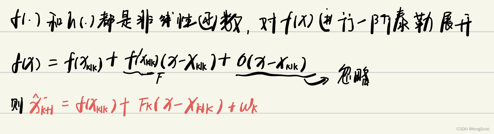
h(?) are nonlinear functions.
Five core formulas of EKF
Motion equation:
x
^
k
+
1
?
=
f
(
x
k
∣
k
)
+
f
‘
(
x
k
∣
k
)
(
x
?
x
k
∣
k
)
+
w
k
\hat{X}^-_{k + 1}=f(x_{k|k}) + f'(x_{k|k})(x-x_{k|k}) + w_k
X^k + 1=f(xk∣k?) + f′(xk∣k?)(x?xk∣k?) + wk?
Covariance matrix:
P
k
+
1
?
=
f
K
P
K
f
K
T
+
Q
k
P_{k + 1}^-=F_KP_KF_K^T + Q_k
Pk + 1=FK?PK?FKT? + Qk?
kalman gain:
K
k
+
1
=
P
k
+
1
?
h
k
+
1
T
(
h
k
+
1
P
k
+
1
?
h
k
+
1
T
+
R
k
+
1
)
?
1
K_{k + 1} =P^-_{k + 1}H^T_{k + 1}(H_{k + 1}P^-_{k + 1}H^T_{k + 1} + R_ {k + 1})^{-1}
Kk + 1?=Pk + 1Hk + 1T?(Hk + 1?Pk + 1Hk + 1T? + Rk + 1?)?1
Status update:
x
^
k
+
1
=
x
^
k
+
1
?
+
K
\hat{X}_{k + 1}=\hat{X}_{k + 1}^- + K
X^k + 1?=X^k + 1 + K
Covariance matrix update:
P
k
+
1
=
P
k
+
1
?
?
K
k
+
1
h
k
+
1
P
k
+
1
?
P_{k + 1}=P^-_{k + 1}-K_{k + 1}H_{k + 1}P^-_{k + 1}
Pk + 1?=Pk + 1?Kk + 1?Hk + 1?Pk + 1
When writing a program, it is a continuous cycle update of Equation 1 to Equation 5.
Matlab implementation of EKF
Now suppose the equation of motion is:
x
k
+
1
=
1
2
x
k
+
2.5
x
k
1
+
x
k
2
+
8
c
o
the s
(
1.2
k
+
w
k
)
X_{k + 1} = \frac{1}{2}X_k + 2.5\frac{X_k}{1 + X_k^2} + 8cos(1.2k + w_k)
Xk + 1?=21?Xk? + 2.51 + Xk2?Xk + 8cos(1.2k + wk?)
Observation equation:
Z
k
=
x
k
2
20
+
v
k
Z_k = \frac{X_k^2}{20} + v_k
Zk?=20Xk2 + vk?
Now calculate the equation of motion for
x
x
The derivative of X is
0.5
+
2.5
1
?
x
2
(
1
+
x
2
)
2
0.5 + 2.5\frac{1-X^2}{(1 + X^2)^2}
0.5 + 2.5(1 + X2)21?X2?
Observation equation pair
x
x
The derivative of X is
x
10
\frac{X}{10}
10X?
They are respectively used as KEF in
f
f
F and
h
h
h
The Matlab code is as follows:
clear;
clc;
T = 100;
Q = 10;w=sqrt(Q)*randn(1,T); % noise in the equation of motion
R = 1;v=sqrt(R)*randn(1,T); % noise in the observation equation
P = eye(1); % covariance matrix

x=zeros(1,T); % store the real state
X=zeros(1,T); % store the predicted state

x(1,1)=0.1; % initial value, the equation of motion needs to determine the state of the next moment according to the previous state
X(1,1)=x(1,1);

z=zeros(1,T); % store observations

for k = 2 : T
    x(:,k) = 0.5 * x(:,k-1) + (2.5 * x(:,k-1) / (1 + x(:,k-1).^2)) + 8 * cos (1.2*(k-1)) + w(k-1);
    z(k) = x(:,k).^2 / 20 + v(k);
    X_ = 0.5*X(:,k-1) + 2.5*X(:,k-1)/(1 + X(:,k-1).^2) + 8 * cos(1.2*(k-1 ));
    F = 0.5 + 2.5 * (1-X.^2)/((1 + X.^2).^2); %The derivative of the motion equation to x is used as F
    H = X_/10; % The observation equation is derived from x as H
    P_=F*P*F' + Q;
    K=P_*H'/(H*P_*H' + R); % calculate kalman gain
    X(k)=X_ + K*(z(k)-X_.^2/20); % update estimated value
    P=P_-K*H*P_; % update covariance matrix
end

% Error Analysis
Xstd=zeros(1,T);
for k=1:T
    Xstd(k)=abs(X(k)-x(k) );
end

figure
hold on; box on;
plot(x,'-ko','MarkerFace','g'); % k indicates that the line is black, o indicates that the data point is a circle, markerface indicates the fill color of the data point, and g indicates that the data point is green
plot(X,'-ks','MarkerFace','b'); % b indicates that the data point is blue
legend('true value','Kalman filter estimated value')
xlabel('time/s');
ylabel('state value x');
figure
plot(Xstd,'-ko');
The execution results are as follows:

The sum(Xstd) calculated this time is 144.5709
When x(1,1) is set to 1, and the initial value of X(1,1) is 0 (that is to say, the initial state estimation is wrong),, the execution results are as follows:

Calculate this sum(Xstd) as 183.1328
Advantages and disadvantages of EKF
advantage:
-
Handling nonlinear systems: EKF can handle a class of nonlinear systems by approximating state transitions and observation models by linearizing nonlinear equations. This makes EKF applicable in many practical problems, because many real-world systems have certain nonlinear characteristics.
-
Efficient implementation: Compared with some more complex nonlinear filtering methods (such as particle filters), EKF has lower computational complexity and higher computational efficiency, especially for small and medium-sized problems.
shortcoming:
-
Sensitive to linearization error: EKF introduces errors when linearizing nonlinear equations, especially for highly nonlinear systems, this linearization error may significantly affect the estimation results. In the case of a high degree of nonlinearity, EKF may produce poor estimation results, and may even diverge.
-
Sensitive to initial estimates: The accuracy of initial state estimates has a greater impact on the performance of EKF. If the initial estimate deviates far from the true state, the EKF may take longer to converge to an accurate estimate.
-
High noise sensitivity: EKF assumes that the system noise is Gaussian white noise. When the system noise is non-Gaussian or the noise is large, the performance of EKF may be affected.
-
Curse of Dimensionality: As the state vector dimension increases, the computational complexity of EKF increases exponentially, which leads to the fact that in high-dimensional problems, EKF may become infeasible or inefficient. This is also a problem that EKF is limited in the application of large-scale or high-dimensional problems.