1. Background introduction
When we are doing data analysis, there are often some outliers in the data. These outliers may be caused by human input errors, instrument failures, or other reasons, but they have a great impact on the final data analysis results. If these outliers are not detected and dealt with in time, it will lead to misjudgment and misleading, which will affect the accuracy of decision-making and results.
Therefore, outlier detection and processing is an indispensable link in the data analysis process. Through effective outlier detection and processing methods, we can eliminate interference factors, improve the accuracy and reliability of data, and conduct data analysis and scientific research more accurately.
This article will introduce the concept of outliers and their impact, the importance of outlier detection and processing, and the experimental principles and implementations of outlier detection and processing. It is hoped that through the introduction of this article, readers can better understand the significance of outlier detection and processing, master the use and operation of related methods, and improve the accuracy and reliability of data analysis.
The content of this issue “Data + Code” has been uploaded to Baidu Netdisk. Friends in need can pay attention to the official account [Xiao Z’s scientific research daily], and reply to the keyword [abnormal value] in the background to obtain.
2. Experimental principles and methods
In the process of data analysis, outlier detection and processing are very important links. In order to help readers better understand the methods and principles of outlier detection and processing, this article will introduce commonly used outlier detection methods, including:
1. IQR method: judge whether the data is an outlier according to the interquartile range of the data.
2. Z-Score method: By calculating the standard deviation and mean of the data, it is judged whether the data deviates from the normal range.
3. Isolation Forest method: Based on the idea of random forest, the data is divided into different subspaces to identify outliers.
4. Local outlier factor method: By calculating the local density around each data point, it is judged whether the data is an outlier.
5. SVM method: Treat the data set as a category, and filter out outliers by predicting the results after training the model.
6. DBSCAN method: classify the data by clustering, and then identify outliers.
The above methods have their own characteristics, and the appropriate method can be selected according to the actual needs for outlier detection and processing. Below I will explain the principle of the above method.
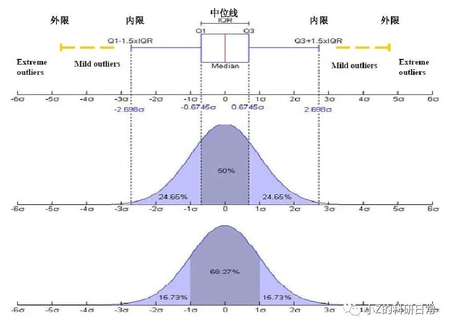
2.1 IQR method
The IQR method is an outlier detection method based on data distribution, and its main idea is to determine the threshold of outliers by calculating the interquartile range (IQR) of the data. Specific steps are as follows:
1. Calculate the first quartile (Q1), second quartile (median), and third quartile (Q3) of the data.
2. Calculate IQR = Q3 – Q1.
3. Determine a constant k (usually 1.5 or 3), and calculate the lower limit lower = Q1 – k * IQR and upper limit upper = Q3 + k * IQR.
4. If a data point is smaller than lower or larger than upper, it is considered an outlier.
Schematic diagram of IQR:

The IQR method is relatively simple and easy to understand, and is often used in scenarios where the data distribution is relatively stable. However, it also has some disadvantages, such as the inability to deal with non-continuous outliers (such as outliers concentrated between two distributions), and the possibility of misjudgment for uneven data distribution.
Q1 = features.quantile(0.25)
Q3 = features.quantile(0.75)
IQR = Q3 - Q1
features = features[~((features < (Q1 - 1.5 * IQR)) |(features > (Q3 + 1.5 * IQR))).any(axis=1)]
2.2 Z-Score method
The Z-Score method is another commonly used outlier detection method. In this method, we calculate the mean and standard deviation of the data and then convert each data point to its Z-Score value. The Z-Score value indicates the degree of deviation of the data point from the mean of the entire data set. The specific steps are as follows:

1. Calculate the mean and standard deviation of the data.
2. For each data point, calculate the degree of deviation from the mean, ie Z-Score = (x – mean) / std.
3. According to the set threshold, judge whether the Z-score value of each data point exceeds the threshold. If exceeded, the data point is considered an outlier.
Among them, x represents the value of the data point, mean represents the mean of the data set, and std represents the standard deviation of the data set. If the Z-Score value of a data point exceeds a preset threshold, it can be considered an outlier.
code show as below:
#Use the Z-Score method to remove outliers
z_scores = np.abs(stats.zscore(features))
features = features[(z_scores < 3).all(axis=1)]
In outlier detection, it is generally considered to be an outlier if it deviates from more than 3 times the standard deviation:

2.3 Isolation Forest Method
Isolation Forest is an anomaly detection algorithm based on tree structure. It divides the sample space into left and right sub-regions by randomly selecting a feature and a segmentation point of the feature, and then recursively divides each sub-region until each sub-region contains only one sample point or reaches a preset maximum depth. Finally, a tree structure with the root node as the starting point and the leaf node as the end point is formed, as shown in the following figure:

Next, we need to calculate the path length of each sample point on this tree, that is, the number of edges passed from the root node to the sample point. The shorter the path length, the greater the difference between the sample point and other sample points, which may be an outlier; otherwise, it is a normal sample.
Finally, we need to set a threshold to judge which sample points are outliers. The usual method is to calculate the average value of the path lengths of all sample points, and if the path length of a certain sample point is smaller than the average value, it is considered an outlier. The specific process is as follows:
1. Randomly select a feature f and a segmentation point v within the value range of the feature from the data set;
2. Divide the data set into left and right subsets, where the left subset contains all samples with feature f less than v, and the right subset contains all samples with feature f greater than or equal to v;
3. If the left subset or the right subset is empty, then terminate the construction of the isolated tree; otherwise, recursively continue to perform steps a) and b) on the left and right subsets until the predetermined tree depth is reached or no further division is possible.
Suppose there are m samples and each sample has n features. For the tth isolated tree, let the sample set be Xt, and construct a binary tree Tt with depth ht. We denote the path length of sample x in Tt by ct(x), which is the number of edges traversed from the root node to x minus 1. According to the algorithm flow, the calculation process of ct (x) can be expressed as follows:

where vti denotes a split point of a randomly selected feature ft in the t-th isolated tree. l and r represent the position of x in the left subtree and right subtree respectively.
isolation_forest = IsolationForest(n_estimators=100, contamination=0.1, random_state=42)
isolation_forest. fit(features)
y_noano = isolation_forest. predict(features)
2.4 Local outlier factor method
The LOF method determines whether each data point is an outlier by calculating the density ratio between it and its neighbors. Specifically, for a data point, if the density of neighbors around it is relatively small, the data point is considered to be an outlier. To use the LOF method to detect outliers, the specific steps are as follows:
1. Choose an appropriate dataset and determine the eigenvectors for each data point.
2. For each data point, calculate its k-nearest neighbors (k-Nearest Neighbors, kNN) set:

where k is a user-defined parameter, usually a small integer.
3. Calculate the Reachability Distance (RD) between each data point and its k-nearest neighbors. The reachable distance represents the distance from the current data point to the furthest point among its k-nearest neighbors.
The larger the reachable distance, the smaller the density between the current data point and its k-nearest neighbors. Define the reachability distance (Reachability Distance) of the i-th data point xi to j as:

Among them, Nk(xj)\{xi} means that xi is excluded from the k-nearest neighbor set of xj, that is, the influence of xi itself is not considered.
4. Define the local outlier factor of the i-th data point as:

where Nk(xi) represents the number of k-nearest neighbors of xi. Computes the local outlier factor (LOF) for each data point. LOF represents the density ratio between the current data point and its k-nearest neighbors. The larger the LOF value, the smaller the density of the current data point relative to its neighbors, and the more likely it is an outlier. Usually, we mark data points with LOF values greater than a certain threshold as outliers.
local_outlier_factor = LocalOutlierFactor(n_neighbors=20, contamination=0.1)
y_noano = local_outlier_factor.fit_predict(features)
2.5 SVM algorithm
The SVM method is an outlier detection based on the distance between the data point and the boundary, assuming we have a training set
X={x1,x2,…,xm}, where each data point is labeled as normal (y=0) or abnormal (y=1). Our goal is to find a decision boundary that separates normal data from abnormal data. The SVM algorithm constructs this boundary by finding a maximum margin hyperplane. A hyperplane is a linear function that partitions the data space, it divides the data into two parts. As shown in the picture:

The implementation steps are as follows:
1. Define the hyperplane: We first define a hyperplane wx + b=0, where w is the normal vector and b is the bias term.
2. Determine the classification rules: For any data point xi, if w.xi + b?0, it will be classified as normal data; otherwise, it will be classified as abnormal data.
3. Maximize interval: After determining the classification rules, we need to find a maximum interval hyperplane that maximizes the distance between normal data and abnormal data. Distances can be calculated using Euclidean distances.
Specifically, for each data point xi, we can calculate its distance to the hyperplane as:

Since we want to maximize the distance, we need to find a hyperplane that maximizes the minimum of all distances ri. This can be formulated as the following optimization problem:

Among them, γ represents the minimum value of the distance.
4. Transform into a dual problem: We transform the optimization problem into a dual problem, and the optimal solution can be obtained more conveniently by solving the dual problem. Specifically, the dual problem is:

Among them, C is a regularization constant and K(xi,xj) is the kernel function. By solving the above optimization problem, the optimal value of α can be obtained.
5. Calculate the normal vector and bias term
The normal vector w and the bias term b can be calculated from the optimal value of α:

6. Detect and handle outliers: After training, you can use it to detect and handle outliers. Specific steps are as follows:
a) Input the new data point x into the model and calculate its distance to the hyperplane:

b) If r exceeds a certain threshold, the data point is marked as an outlier; otherwise, it is marked as normal data.
one_class_svm = OneClassSVM(nu=0.1, kernel='rbf', gamma=0.1)
y_noano = one_class_svm.fit_predict(features)
2.6 DBSCAN algorithm
DBSCAN determines cluster boundaries by calculating the density between data points, and treats data points that do not belong to any cluster as anomalies.
Its principle is to find high-density regions and divide these regions into a cluster. Specifically, for each data point, the algorithm counts the number of points in its neighborhood within its radius ε, and if the number of points exceeds the threshold MinPts, the point is considered a core point. Then, starting from the core point, the algorithm expands the cluster along the density-reachable path until no new points can be added.
If a data point is not a core point, but is in the neighborhood of a core point, then it is classified as the cluster where the core point is located. Otherwise, the data point is considered noise or an outlier. Specific steps are as follows:
1. Randomly select an unvisited data point p.
2. If the number of points in the neighborhood of p is less than MinPts, mark p as a noise point.
3. Otherwise, create a new cluster C and add p to C.
4. For each data point q within the neighborhood of p: a. If q is not visited, mark it as visited and join C b. If q is a core point, recursively process the data points within its neighborhood.
5. Repeat steps 1-4 until all points have been visited.

Now let’s derive the core formula of the DBSCAN algorithm. Suppose there is a data set D={x1,x2,…,xn}, where each data point xi has a density ρi. We define the density within the radius ε as:

Among them, I( ) is an indicator function, which outputs 1 if the condition in the brackets is true, otherwise it outputs 0. That is, ρi is the number of points that are no more than ε away from xi.
Next, we define the reachable distance δ(p,q) of a data point xi, which represents the shortest distance from p to reach q along the density reachable path. Specifically, for any two data points p and q, their reachable distance is:

Among them, NMinPts(q) represents the set of core points contained in the neighborhood with q as the center and radius ε.
Finally, we define a local outlier factor LOF(xi) for a data point xi, which represents the ratio of its density to the density of surrounding points:

The performance of the DBSCAN algorithm is relatively sensitive, and it is necessary to adjust the parameters to obtain better clustering results. Specifically, it is necessary to set an appropriate radius ε and the minimum number of points MinPts in the neighborhood. If ε is too small, noise points will be mistaken as part of a cluster; if ε is too large, different clusters will be merged together. Likewise, if MinPts is too small, too many clusters will be produced; if MinPts is too large, it will cause many data points to be considered noise.
dbscan = DBSCAN(eps=0.5, min_samples=10)
y_noano = dbscan. fit_predict(features)
3. Experimental results display
This experiment uses the Boston house price data set to realize the effect of different methods for outlier detection through Python. First analyze by plotting a violin plot on the raw data:
Through the violin plot, it can be clearly observed that the Dis and Ptratio features have many outliers. The following will visualize the distribution of data after removing outliers by different methods, and compare the distribution of eigenvalues before and after removing outliers by different methods.

As can be seen from the above two figures, no matter which method, the features are concentrated in the 0-5 area. After using the IQR method, Z-Score method and Isolation Forest method to remove outliers, some discrete points appeared within 5-80 to make each feature mean; while using the local outlier factor method, single-class SVM method and DBSCAN method After removing outliers, the data distribution becomes more concentrated, but there are still some outliers. In addition, it can also be seen that before and after using the IQR method to remove outliers, the standard deviation and range of the data are significantly reduced, indicating that this method can effectively reduce the degree of abnormality of the data.
Then, we can further use the box plot to observe the data distribution after different methods remove outliers. As follows:

As can be seen from the figure above, after using the local outlier factor method, the one-class SVM method and the DBSCAN method to remove outliers, the data distribution becomes tighter, but there are still some outliers far away from the main body. However, after using the IQR method, Z-Score method and Isolation Forest method to remove outliers, the data distribution is relatively uniform, and the outliers are significantly reduced.
The final results show that different methods may produce different results, so you need to choose the method that is most suitable for your data set in practical applications. At the same time, when performing outlier detection and cleaning, it is also necessary to select and adjust according to the specific situation.
Thank you for reading this article! If you are interested in data analysis and outlier detection methods, please pay attention to our WeChat public account (Xiao Z’s scientific research daily).