Table of Contents
1. Basic principles of ant colony optimization algorithm
1.1 Pheromone update formula
1.2 Ant selection path formula
1.3 Cost function formula
1.4. Constraint condition processing formula
2. Ant colony optimization algorithm matlab program
3. Simulation results
1. Basic principles of ant colony optimization algorithm
Ant colony optimization algorithm is a heuristic optimization algorithm that solves some combinatorial optimization problems by simulating the behavior of ants in nature looking for food. In the VRP (Vehicle Routing Problem) path planning problem, the ant colony optimization algorithm can be used to find the shortest or optimal path so that a certain number of vehicles can meet customer needs at the lowest cost. The basic principles of the ant colony optimization algorithm are:
When ants are looking for food, they will leave pheromones on the path. Subsequent ants will choose a path based on the strength of the pheromone, and the pheromones will evaporate over time. Therefore, ants will find the shortest path from the food source to the ant nest in the process of volatilizing and accumulating pheromones.
In the VRP path planning problem, the driving path of each vehicle can be regarded as a segment of sub-paths. Each sub-path has a certain length and cost, and the ants need to leave pheromone on this sub-path. When subsequent ants choose paths, they will give priority to sub-paths with high pheromone intensity, short length, and low cost. Through continuous iteration and optimization, a set of optimal sub-paths can finally be obtained to form a complete vehicle driving path.
1.1 Pheromone Update Formula
The pheromone update formula is one of the cores of the ant colony optimization algorithm. At time t, the pheromone concentration left by the i-th ant on the j sub-path is τ(t), and its update formula is:
τ(t + 1) = (1 – ρ) × τ(t) + ρ × Δτ(t)
Among them, ρ is the pheromone volatilization rate, (1 – ρ) is the persistence factor of the pheromone; Δτ(t) is the pheromone increment left by the i-th ant on the j sub-path at time t, and its calculation formula for:
Δτ(t) = Q / L(t)
Among them, Q is the total amount of pheromone, and L(t) is the length of the path taken by the i-th ant at time t.
1.2 Ant selection path formula
At time t, the probability P^(k)ij(t) of the k-th ant choosing the j sub-path is:
P^(k)ij(t) = (τ(t))^α / Σ_l ((τ(t))^α)
Among them, α is the pheromone importance factor, which determines the sensitivity of ants to pheromone; Σ_l ((τ(t))^α) is the sum of the pheromone importance on all sub-paths.
1.3 Cost function formula
The cost function formula is used to measure the quality of each sub-path. For a fixed sub-path j, its total cost C^(j) can be expressed as:
C^(j) = c1 × L^(j) + c2 × (N^(j) – 1)
Among them, L^(j) is the length of sub-path j; N^(j) is the number of customers on sub-path j; c1 and c2 are fixed cost coefficients. For the entire vehicle travel path, its total cost C can be expressed as:
C = Σ_j (C^(j)) / J
Among them, J is the total number of trains. The goal is to minimize C.
1.4. Constraint condition processing formula
The load capacity of each vehicle cannot exceed its maximum load capacity, and the driving distance of each vehicle cannot exceed its maximum driving distance. These two constraints can be handled by the penalty function method. For load capacity constraints, a load capacity penalty function P_weight can be introduced:
P_weight = max(0, W – w)
Among them, W is the maximum load capacity of the vehicle, and w is the actual load capacity of the current vehicle. Similarly, a driving distance penalty function P_distance can be introduced:
P_distance = max(0, D – d)
Among them, D is the maximum driving distance of the vehicle, and d is the actual driving distance of the current vehicle. Finally, add these two penalty functions to the cost function:
C = Σ_j (C^(j)) / J + Σ_k (P_weight + P_distance) / K
Among them, K is the total number of vehicles. The goal is to minimize C.
2. Ant colony optimization algorithm matlab program
........................................................ .........
D=Distanse(C);
%Construct savings matrix
U=zeros(n,n);%U represents the connection between factories and the distance that can be saved by the connection with the warehouse
for i=1:n
U(i,i)=eps;
for j= 1:n
U(i,j)=D(i,1) + D(j,1)-D(i,j);
U(j,i)= U(i,j);
end
end
U=U + 1;
load_w=0;
Eta=1./D;%Eta is the heuristic factor, here it is set as the reciprocal of distance
Tau=ones(n,n);%Tau is the pheromone matrix
Tabu=zeros(m,n + 4);% store and record path generation
NC=1;% iteration counter
G_best_route=[NC_max,n + 4];%The best route of each generation
G_best_length=inf.*ones(NC_max,1);%The length of the best route of each generation
length_ave=zeros(NC_max,1);%The average length of each generation route
Obj=zeros(NC_max,1);
%%The second step is to put the ants into the DC
while NC<=NC_max%One of the stopping conditions: the maximum number of iterations is reached
Tabu(:,1)=ones(m,1);
%%The third step, m ants select the factory according to the required method and complete the tour
for i=1:m
for j=2:n + 4
visited=Tabu(i, :);
visited=visited(visited>0);
to_visit=setdiff(1:n,visited);
x=zeros(length(to_visit),1);
if isempty(to_visit) % Select the next factory according to the rules or return to the warehouse
Tabu(i,length(visited) + 1)=1;
load_w=0;
continue;
end
for k=1:length(to_visit)
x(k)=(Tau(visited(end),to_visit(k))^Alpha)*(Eta(visited(end),to_visit(k))^Beta);%*(U(visited(end),to_visit (k))^gama);
end
if rand<qq
Select=find(max(x));
else
x=x/(sum(x)); %Select the next city based on the principle of probability
xcum=cumsum(x);
Select=find(xcum>=rand,1,'first');
end
load_w=load_w + t(to_visit(Select));
if load_w>W
load_w=0;
Tabu(i,length(visited) + 1)=1;
else
Tabu(i,length(visited) + 1)=to_visit(Select);
end
end
end
%% The fourth step records various parameters of this generation.
L=zeros(m,1);
for i=1:m
MM=Tabu(i,:);
R=MM(MM>0);
for j=1:(length(R)-1)
L(i)=L(i) + D(R(j),R(j + 1));
end
end
[G_best_length(NC),pos]=min(L);
G_best_route(NC,1:length(Tabu(pos(1),:)))=Tabu(pos(1),:);
%%Apply the 2-opt method to update the optimal solution
select=find(G_best_route(NC,:)==1);
FF=[];%Record new route
LM=0;% calculate new value
for a=1:(length(select)-1)
y_G_best_route=G_best_route(NC,select(a):select(a + 1));%Select the first route
al=length(y_G_best_route);
T=zeros((length(select)-1),1);% record the length of each route
% Calculate the length of each route
for d=1:(al-1)
T(a)=T(a) + D(y_G_best_route(d),y_G_best_route(d + 1));
end
for b=2:(al-1)
for c=(b + 1):(al-1)
DD=y_G_best_route;
% swap positions
temp1=DD(b);
temp2=DD(c);
DD(b)=temp2;
DD(c)=temp1;
% record distance
TT=zeros(1);
for d=1:(al-1)% calculates the distance after swapping positions
TT=TT + D(DD(d),DD(d + 1));
end
if TT<T(a)
T(a)=TT;
y_G_best_route=DD;
end
end
end
if a>=2
y_G_best_route=y_G_best_route(2:al);
end
%Update route and length
FF=[FF,y_G_best_route];
LM=LM + T(a);
end
%Update optimal route and length
................................................................. .............................
end
%%Step 7: Output the results
[best_length,Pos]=min(G_best_length);
best_route=G_best_route(Pos(1),:);
best_route=best_route(best_route>0);
disp(best_route);
disp('The minimum stroke is:')
disp(best_length);
toc
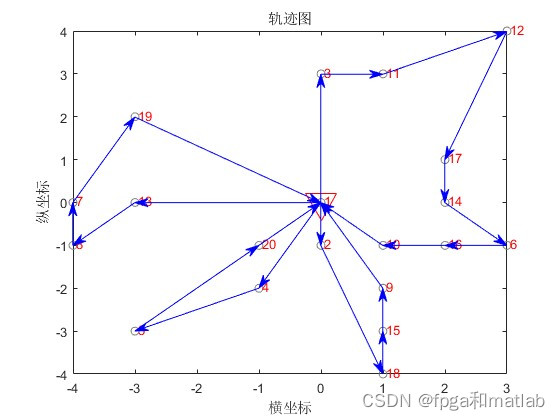
%% Path diagram of optimal solution
DrawPath(best_route(1:end-1),C)
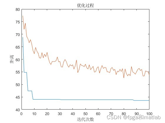
%% Optimization process iteration diagram
figure
plot(1:NC_max,Obj)
hold on
plot(length_ave)
xlabel('Number of iterations')
ylabel('distance')
title('Optimization process')
up2257
3. Simulation results
The knowledge points of the article match the official knowledge files, and you can further learn related knowledge. Algorithm skill tree Home page Overview 57368 people are learning the system