[Pytorch] derivative and derivation

Article directory

Derivatives and Derivatives
- 1. Derivatives of scalar vector matrix
- 2. Reverse derivation in Pytorch.backward()
- 3. Non-scalar derivation

Derivatives and derivatives

1. Derivative of scalar vector matrix

Shape after differentiation between scalars, vectors, and matrices:

y\x	scalar x(1)	vectorx(n,1)	matrixX(n,k)
scalar y(1)	(1)	(1,n)	(k,n)
Vectory< /strong>(m,1)	(m,1)	(m,n)	(m,k,n)
MatrixY(m,l)	(m,l)	(m,l,n)	(m,l,k,n)

and

In the case of vectors:

< x , w >

When x and w are vectors: \frac{?<\bm x ,\bm w>}{?\bm w} = \bm x^{T}

When x and w are vectors: ?w??=xT

is the matrix

In the case of vectors:

When x is a matrix w is a vector: \frac{?\bm {X w}}{?\bm w} = \bm X

When x is a matrix w is a vector: ?w?Xw?=X

special,

the s

Indicates when summing vector elements:

In particular, sum means when summing vector elements:

In the case of vectors:

the s

yes and

the same shape

the vector

When x is a vector: \frac{?\bm x.sum}{?x} = \bm1\space\space where \bm1 is a full 1 vector with the same shape as x

When x is a vector: ?x?x.sum?=1 where 1 is a vector of all 1s with the same shape as x

2. Reverse derivation in Pytorch.backward()

Reverse derivation in Pytorch is implemented with the .backward() method

y.backward()

x = torch.arange(4.0)
x. requires_grad_(True)
y = torch.tensor([3.0, 1.0, 2.0, 5.0], requires_grad=True)
z = 2 * torch.dot(x, y)
print(x, '\\
', y, '\\
', z)
print("Backpropagation:")
z. backward()
print(f"z partial derivative of x: {<!-- -->x.grad}")
print(f"Partial derivative of z to y: {<!-- -->y.grad}")
y.grad.zero_()
z = y. sum()
z. backward()
print(f"Derivative of y.sum to y: {<!-- -->y.grad}")

3. Non-scalar derivation

For the case of vector differentiation:

The derivative of vector y with respect to vector x is a Jacobian matrix, which is usually obtained in deep learning as a square matrix

Suppose X = [x1, x2, x3, x4] ; Y = [y1, y2, y3, y4], where

the y

{y_i}={x_i}^2

yi?=xi?2, then the derivative of Y to X can be expressed as the Jacobian determinant:

However, the output of the backward() method in pytorch needs to be a tensor of the same dimension as the original tensor, so when encountering vector derivation, an additional parameter gradient must be passed in backward, and the gradient is a shape of the same shape as Y Tensor, used to multiply the Jacobian determinant to the left to obtain the final derivative with the same shape as Y:

In addition to using the backward() method in the form of passing parameters, you can also use the .sum() method:

y.sum().backward() #The effect is equivalent to y.backward(torch.ones_like(y)

x = torch.tensor([1, 2, 3, 4], requires_grad=True, dtype=float)
y = torch. tensor([3, 4, 5, 6], requires_grad=True, dtype=float)
z = x * y
z. sum(). backward()
print(x.grad)

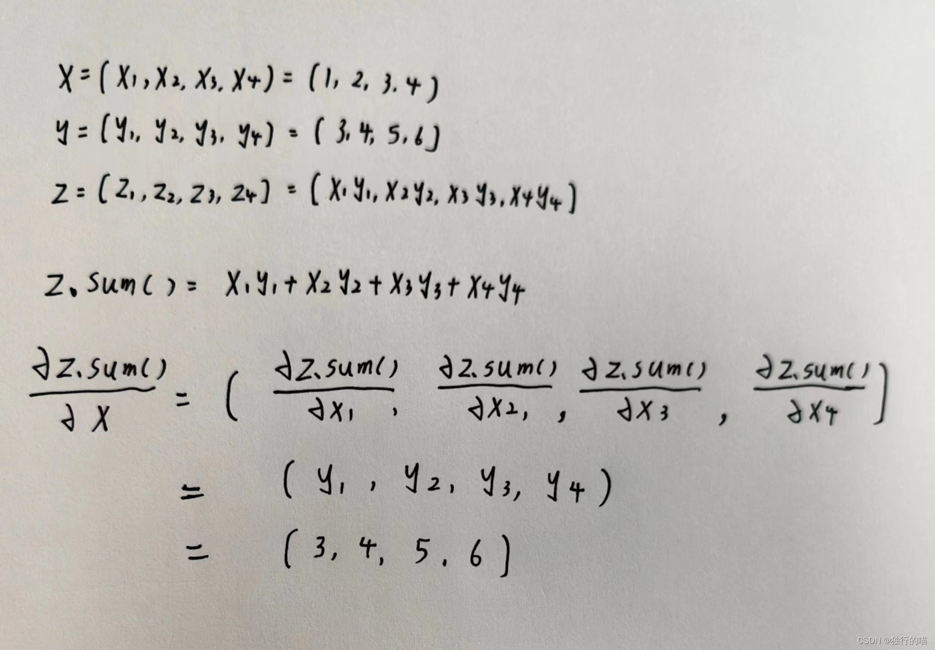
Mathematical explanation about derivation using the .sum() method:

Several code examples of vector derivation are as follows:

import torch


# Define vectors x and y, and the operation result z is also a vector
x = torch.tensor([1, 2, 3, 4], requires_grad=True, dtype=float)
y = torch. tensor([3, 4, 5, 6], requires_grad=True, dtype=float)
z = x * y
print('z:', z)

# 1. Perform reverse derivative on the vector z, and the input parameter is the ones vector with the same shape as z
z.backward(torch.ones_like(z), retain_graph=True)
print(x.grad)

# 2. Change the parameter to a vector of the same shape as z [2, 3, 4, 5] and reverse the derivative again
x.grad.zero_()
z.backward(torch.tensor([2, 3, 4, 5]).reshape(z.shape), retain_graph=True)
print(x.grad)

# 3. Use the .sum() function to process vector derivation, the effect is equivalent to 1: z.backward(torch.ones_like(z)
x.grad.zero_()
z. sum(). backward()
print(x.grad)

operation result:

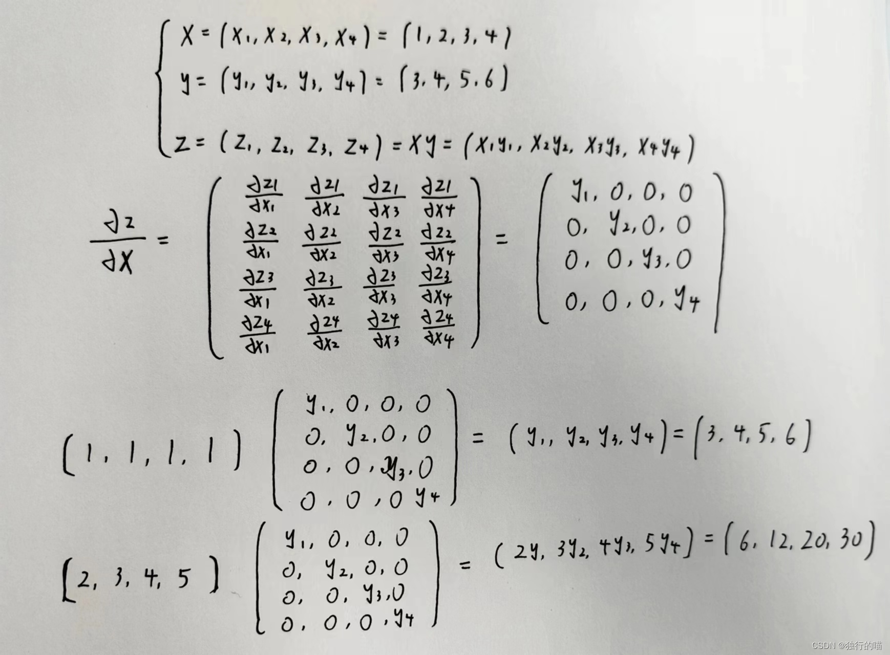
The result after using the .sum method to assist the derivation is [3, 4, 5, 6], which is equivalent to multiplying the row vector [1, 1, 1, 1] to the left of the Jacobian determinant and the result is: [ 3, 4, 5, 6]
After changing the parameters in the backward() method to [2, 3, 4, 5], it is equivalent to multiplying the original Jacobian determinant by the row vector [2, 3, 4, 5] to the left, which should be in the original result On the basis of [3, 4, 5, 6], multiply each line by 2, 3, 4, 5 respectively, and the final result is [6, 12, 20, 30]

Reference blog post:
https://blog.csdn.net/qq_52209929/article/details/123742145
https://zhuanlan.zhihu.com/p/216372680