An older technology, but still learn to understand.
Vector Quantization (VQ)
Vector quantization is a signal compression method and a lossy compression method based on block coding rules. This technique is widely used in the fields of signal processing and data compression. In fact, there are VQ steps in multimedia compression formats such as JPEG and MPEG-4.
Introduction
The name Vector Quantization sounds a bit mysterious, but it is not so profound in itself. Everyone knows that analog signals are continuous values, and computers can only process discrete digital signals. When converting analog signals to digital signals, we can use a certain value in the interval to replace an interval, for example, [ All values on 0, 1) become 0, all values on [1, 2) become 1, and so on. In fact, this is a VQ process. A more formal definition is: VQ is the process of encoding points in a vector space with a finite subset of them.
Principle
That is, the conversion of continuous information into digital signals.
Basic idea:
Several scalar data groups are formed into a vector, and then quantized as a whole in the vector space, thereby compressing the data without losing much information.

VQ is actually a kind of approximation: using a number to approximate the numbers around it; for example, rounding in mathematics? x ?
Example
One-dimensional example:
VQ is actually an approximation. Its idea is similar to that of “rounding”. It uses an integer that is closest to a number to approximate the number.
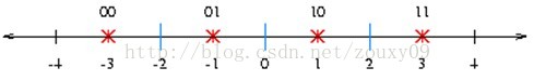
Here, numbers less than -2 are approximately -3, numbers between -2 and 0 are approximately -1, numbers between 0 and 2 are approximately 1, and numbers greater than 2 are approximately 3. In this way, any number will be approximated as one of the four numbers -3, -1, 1 or 3. And we only need two binary bits to encode these four numbers. So this is 1-dimensional, 2-bit VQ, and its rate (quantization rate?) is 2bits/dimension.
2D example:
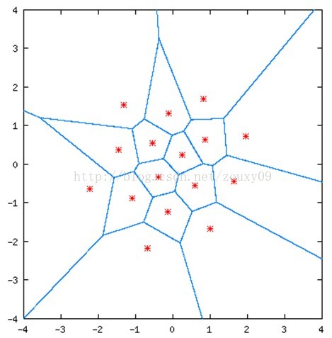
In the picture above, the solid blue line divides the picture into 16 areas, each with a red star point; any coordinate will fall into a specific area in the picture above. It will then be approximated by the point of the red star in the area.
These red star points are quantized vectors, which means that any point in the graph can be quantized as one of these 16 vectors. That is, these 16 red star points can describe the whole picture.

Then these 16 values can be encoded with 4-bit binary code (2^4=16). Therefore, this is a 2-dimensional, 4-bit VQ, and its rate is also 2bits/dimension.
Image encoding example:
In the simplest case, consider a grayscale image, 0 is black, 1 is white, and the value of each pixel is a real number on [0, 1]. Now to encode it into a 256-level grayscale image, the simplest way is to map each pixel value x to an integer floor(x255) . Of course, the original data space does not have to be continuous. For example, now you want to compress this picture, each pixel is stored using only 4 bits (instead of the original 8 bits), therefore, you need to use [0, 15] for the original integer value on the interval [0, 255] ] to encode integer values on ], a simple mapping scheme is x15/255.
However, such a mapping scheme is quite naive. Although it can reduce the number of colors to achieve a compression effect, if the original colors are not evenly distributed, the quality of the resulting image may not be very good. For example, if a 256-level grayscale image consists entirely of two colors, 0 and 13, then the above mapping will result in a completely black image because both colors are mapped to 0. A better approach is to combine clustering to select representative points.
The actual method is: treat each pixel as a piece of data, run K-means to get k centroids, and then use the pixel values of these centroids to replace the pixel values of all points in the corresponding cluster. For color pictures, the same method can be used, such as RGB three-color pictures, each pixel is regarded as a point in a 3-dimensional vector space.
The three pictures of VQ 2, VQ 10 and VQ 100 show the results obtained when the number of clusters is 2, 10 and 100 respectively. It can be seen that VQ 100 is very close to the original picture. After replacing many of the original color values with centroids, the total number of colors is reduced, and the number of repeated colors is increased. This kind of redundancy is what the compression algorithm likes most. Consider one of the simplest compression methods: store the color information of centroids separately (for example, 100), and then store the centroid index instead of the color information value for each pixel. If an RGB color value requires 24 bits to store, each The index value (within 128) only needs 7 bits to store, which has the effect of compression.
The original image:

VQ2:

VQ 10:

VQ100:

code:
The kmeans and vq functions provided by SciPy are directly used, and the Python Image Library is used for image reading and writing.
#!/usr/bin/python

from scipy.cluster.vq import kmeans, vq
from numpy import array, reshape, zeros
from mltk import image

vqclst = [2, 10, 100, 256]

data = image.read('example.jpg')
(height, width, channel) = data. shape

data = reshape(data, (height*width, channel))
for k in vqclst:
    print 'Generating vq-%d...' % k
    (centroids, distor) = kmeans(data, k)
    (code, distor) = vq(data, centroids)
    print 'distor: %.6f' % distor.sum()
    im_vq = centroids[code, :]
    image.write('result-%d.jpg' % k, reshape(im_vq,
        (height, width, channel)))
Of course, Vector Quantization does not have to be done with K-means, all kinds of clustering methods can be used, but K-means is usually the simplest, and usually enough.
Description of mathematical formula
-
Suppose a training sequence (training set) with M vector sources (training samples): T={x1, x2,…, xM};
-
Assuming each source vector is k-dimensional:
xm=(xm1,xm2, …, xmk), m=1,2,…,M -
Assuming that the number of code vectors is N (that is, we need to divide this vector space into N parts, or quantize it into N values), the codebook (the set of all code vectors) is expressed as: C={c1, c2, …, cN};
-
Each code vector is a k-dimensional vector: cn=(cn1, cn2, …, cnk), n=1, 2, …, N;
-
The coding region corresponding to the code vector cn is denoted as Sn, and then the division of the space is expressed as:
P={S1, S2,…,SN};
If the source vector xm is within Sn, then its approximation (denoted by Q(xm)) is cn,
Q(xm)=cn.
Assuming that we use the average error distortion measure, then the average distortion degree is expressed as follows (using Euclidean distance):
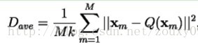
Then the design problem can be simply described as:
Given T (training set) and N (number of code vectors), find C (codebook) and P (space partition) that minimize Dave (average distortion).
Optimization Criteria:
If C and P are a solution to the minimization problem above, then the solution needs to satisfy the following two conditions:
(1) Nearest NeighborCondition nearest neighbor condition:
 This condition means that the encoding region Sn should contain all the vectors closest to cn (compared to distances of other codevectors). For vectors above the boundary (blue line), any tie-breaking procedure is required.
(2) Centroid Condition centroid condition:
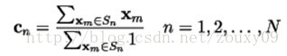
This condition requires that the code vector cn is the average vector of all training sample vectors in the coding region Sn. In the implementation, it is necessary to ensure that each coding region has at least one training sample vector, so that the denominator of the above formula is not 0.
LBG algorithm
LBG