No framework, just use numpy to write a wonderful chapter of DNN (Deep Neural Networks)

1. Overview

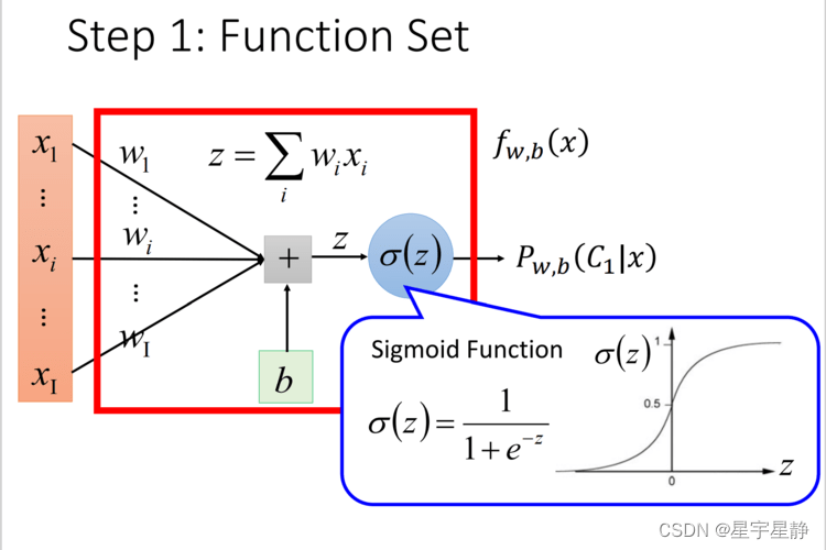
A Logistics Regression can be thought of as a simple neural network consisting of only one hidden layer (Hidden Layer) (as shown in the figure below).

However, Logistic Regression is often very sensitive to outliers, and it is difficult to deal with polyphenols. Therefore, people were inspired by human brain nerves and established more complex neural networks with more layers based on Logistic Regression. Model, also called Deep Neural Networks (DNN)

Deep neural networks have revolutionized machine learning and turned it into deep learning. People feel scary when they hear deep learning, but I want to say that after reading the writing of DNN code below, you will find that deep learning is actually not that difficult.

2. Basic principles

Figure 2 Neural network with two hidden layers

As shown in the figure, there is a seemingly complex network structure. Its input is a vector with three features. The output can be considered as a logistic regression classifier with two hidden layers in the middle. As shown in the figure, we combine all The layers are numbered $l_i$ , where Input Layer is As $l_0$ Output Layer as $\$ . According to the basics of logistic regression, we should design a forward network and a backward network to calculate respectively $\hat{y_i}$ and gradient grad. As shown below

3. Code implementation

Initialization parameters

First we need to initialize our parameter param ( $w_i, b_i$ ), so we design an initialization function:

def init_param(dim, m):
    param = {}
    L = len(dim)
    for i in range(1, L):
        param["W" + str(i)] = np.random.randn(dim[i], dim[i - 1])
        param["b" + str(i)] = np.random.randn(dim[i], m)

    return param

The input of this function is dim, which is the dimension of each layer of the network. For example, the input in Figure 2 should be [3, 4, 3, 1], and m is the amount of data.

Activation function and derivative of activation function

import numpy as np


def sigmoid(Z):
    g = 1.0 / (1.0 + np.exp(-1.0 * Z))

    return g


def d_sigmoid(Z):
    s = 1.0 / (1.0 + np.exp(-1.0 * Z))
    dg = s * (1-s)

    return dg

Here we take the sigmoid function as an example. If you need to use other activation functions, just add a logo recognition. It is worth noting here that the derivative calculation of the sigmoid function can be expressed as dg = s * (1-s) according to the Stanford University Open Course, where s is the original function.

Forward propagation

Since there are many levels, we need to calculate the output of forward propagation one by one. The relationship between each step is

where< img alt="n_l" class="mathcode" src="//i2.wp.com/latex.csdn.net/eq?n_l">is the $l$ The dimension of the layer, the number in brackets is the dimension, we can use this dimension to The code is inspected.

def forward(A, param):
    cache1 = [A]
    cache2 = []

    L = len(param) // 2

    for i in range(1, L + 1):
        Z = np.dot(param["W" + str(i)], A) + param["b" + str(i)]
        A = sigmoid(Z)
        cache2.append(Z)
        cache1.append(A)
    cache = cache1, cache2

    return A, cache

The input A here is the initial input latex.csdn.net/eq?w_i, b_i”>), the parma here is stored in the form of a dictionary. The storage method can be seen from the for loop.

When outputting, I retained the A used in the next cost function = $\hat{y}$ , and also retains part of the data in the cache to speed up subsequent reverse propagation.

Cost function

The general cost function is calculated using cross entropy, as follows

$Loss = -\frac{1}{m}[ylog\hat{y} + (1-y)log(1-\hat{y})]$

The corresponding code is as follows:

def cost(A, y):
    m = y.shape[1]
    J = -(1.0 / m) * np.sum(y* np.log(A) + (1-y)*np.log(1-A))

    return J

The A entered here is $\hat{y}$ But for the sake of unification, I will call it A.

Backpropagation

Because backpropagation involves the broadcast mechanism of python, it is more troublesome to think about. In fact, the general form of backpropagation of the lth hidden layer can be obtained by derivation of the composite function and finding the rules.

The specific code is as follows:

def backward(y, cache, param):
    grad = {}
    A, Z = cache
    L = len(param) // 2

    dZ = A[L]-y
    grad["dW" + str(L)] = np.dot(dZ, A[L - 1].T) / m
    grad["db" + str(L)] = np.sum(dZ) / m
    for i in range(L-1, 0, -1):
        dA = np.dot(param["W" + str(i + 1)].T, dZ)
        dg = d_sigmoid(Z[i - 1])
        dZ = dA * dg
        grad["dW" + str(i)] = np.dot(dZ, A[i - 1].T) / m
        grad["db" + str(i)] = np.sum(dZ) / m

    return grad

Input the target value y, cache, parameter param, and return a gradient grad.

Update parameters

This part is relatively simple, the formula is as follows:

$W_l = W_l - \alpha dW_l$

$b_l = b_l - \alpha db_l$

code show as below:

def update_param(param, grad, alpha):
    L = len(param) // 2

    for i in range(1, L):
        param["W" + str(i)] -= alpha * grad["dW" + str(i)]
        param["b" + str(i)] -= alpha * grad["db" + str(i)]

    return param

Integrate model

def train(X, Y, layer_dim, alpha, epochs):
    m = X.shape[1]
    param = init_param(layer_dim, m)
    for i in range(epochs):
        A, cache = forward(X, param)
        J = cost(A, Y)
        grad = backward(Y, cache, param)
        update_param(param, grad, alpha)
        print(J)

    return J, param

Put all the functions into the training function to form a model.

The knowledge points of the article match the official knowledge archives, and you can further learn relevant knowledge. Python introductory skill treeScientific computing basic software package NumPyNumPy overview 388,937 people are learning the system