1.Experimental purpose:
Understand the principle of K-means algorithm and use K-means algorithm to implement iris clustering.
2.K-meansIntroduction to the algorithm
Clustering is a process of classifying and organizing data members that are similar in some aspects of the data set. Clustering is a technique for discovering this inherent structure. Clustering technology is often called unsupervised learning. K-means clustering is the most famous partitioning clustering algorithm. Due to its simplicity and efficiency, it has become the most widely used among all clustering algorithms. Given a set of data points and the required number of clusters k, where k is specified by the user, the k-means algorithm repeatedly divides the data into k clusters based on a certain distance function.
3.K-meansAlgorithm principles and steps
The K-means algorithm is a typical clustering algorithm based on distance (Euclidean distance, Manhattan distance). It uses distance as the evaluation index of similarity, that is, it is considered that the closer the distance between two objects, the greater the similarity. This algorithm believes that clusters are composed of objects that are close together, so it takes the ultimate goal of obtaining compact and independent clusters.
Algorithm steps:
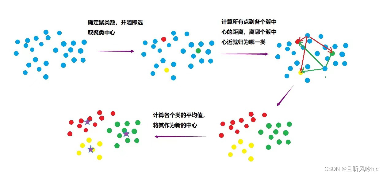
- First define how many clusters there are in total, and randomly select K samples as cluster centers.
- Calculate the distances from all samples to the randomly selected K cluster centers.
- The sample is assigned to which cluster center is closest to the center.
- Calculate the mean of each center sample (the simplest method is to find the mean of each point of the sample) as the new cluster center.
- Repeat 2, 3, and 4 until the new center is basically unchanged from the original center, and the algorithm ends.
Algorithm end condition:
k-menas can be stopped when the centroid of each cluster no longer changes. When the number of cycles reaches the predetermined number, k-means is stopped.
Principle diagram:
K-means flow chart:

Euclidean distance calculation formula: The Euclidean distance between points x= (x_1,x_2,…,x_n) and y= (y_1,y_2,…,y_n) is:

Manhattan distance: The Manhattan distance between points x= (x_1,x_2,…,x_n) and y= (y_1,y_2,…,y_n) is:
![]()
Cluster center update formula: During each iteration, we need to update the center of each cluster. Assuming that the data points contained in cluster C are x(1), x(2)…x(m), then the center of cluster C can be obtained by calculating the mean of all data points in the cluster:

4.Iris data analysis
1) Contains 3 data types, a total of 150 pieces of data
2) Contains 4 features: sepal length, sepal width, petal length, and petal width.
5.Experimental Tools
Windows 11, PyCharm.
6.Code Implementation
import matplotlib.pyplot as plt
import numpy as np
from sklearn.cluster import KMeans
from sklearn import datasets

# Get the data set directly from sklearn
iris = datasets.load_iris()
X = iris.data[:, :4] # means we take 4 dimensions in the feature space
print(X.shape)

# Take the first two dimensions (sepal length, sepal width) and draw the data distribution chart
plt.scatter(X[:, 0], X[:, 1], c="red", marker='o', label='see')
plt.xlabel('sepal length')
plt.ylabel('sepal width')
plt.legend(loc=2)
plt.show()

def Model(n_clusters):
    estimator = KMeans(n_clusters=n_clusters)# Construct clusterer
    return estimator

def train(estimator):
    estimator.fit(X) # Clustering

# Initialize the instance and start training fitting
estimator=Model(3)
train(estimator)

label_pred = estimator.labels_ # Get clustering labels
# Plot k-means results
x0 = X[label_pred == 0]
x1 = X[label_pred == 1]
x2 = X[label_pred == 2]
plt.scatter(x0[:, 0], x0[:, 1], c="red", marker='o', label='label0')
plt.scatter(x1[:, 0], x1[:, 1], c="green", marker='*', label='label1')
plt.scatter(x2[:, 0], x2[:, 1], c="blue", marker=' + ', label='label2')
plt.xlabel('sepal length')
plt.ylabel('sepal width')
plt.legend(loc=2)
plt.show()


# Euclidean distance calculation
def distEclud(x, y):
    return np.sqrt(np.sum((x - y) ** 2)) # Calculate Euclidean distance
# Construct a set of K random centroids for the given data set
def randCent(dataSet, k):
    m, n = dataSet.shape # m=150,n=4
    centroids = np.zeros((k, n)) # 4*4
    for i in range(k): # Execute four times
        index = int(np.random.uniform(0, m)) # Generate random numbers from 0 to 150 (randomly pick a vector in the data set as the initial value of the centroid)
        centroids[i, :] = dataSet[index, :] # Pass the four dimensions of the corresponding row to the set of centroids
    return centroids
# k-means clustering algorithm
def KMeans(dataSet, k):
    m = np.shape(dataSet)[0] # Number of rows 150
    # The first column stores which cluster each sample belongs to (four clusters). The second column stores the error of each sample to the center point of the cluster.
    clusterAssment = np.mat(np.zeros((m, 2))) # .mat() creates a 150*2 matrix
    clusterChange=True
    # 1. Initialize centroids
    centroids = randCent(dataSet, k) # 4*4
    while clusterChange:
        # Stop iteration when the cluster to which the sample belongs is no longer updated
        clusterChange = False
        # Traverse all samples (number of rows 150)
        for i in range(m):
            minDist = 100000.0
            minIndex = -1
            # Traverse all centroids
            # 2. Find the nearest centroid
            for j in range(k):
                # Calculate the Euclidean distance between the sample and the four centroids and find the nearest centroid minIndex
                distance = distEclud(centroids[j, :], dataSet[i, :])
                if distance < minDist:
                    minDist=distance
                    minIndex = j
            # 3. Update the cluster to which the row sample belongs
            if clusterAssment[i, 0] != minIndex:
                clusterChange=True
                clusterAssment[i, :] = minIndex, minDist ** 2
        # 4. Update centroid
        for j in range(k):
            # np.nonzero(x) returns the subscript of the element whose value is not zero. Its return value is a tuple with length x.ndim (number of axes of x)
            # Each element of the tuple is an integer array, and its value is the value of the subscript of the non-zero element on the corresponding axis.
            #Matrix name.A represents converting the matrix into array array type

            #Here, take the first column of all rows of the matrix clusterAssment, convert it into an array, compare it with j (cluster label value), and return true or false
            # Generate an array through np.nonzero, which is the subscript value (x) of all points corresponding to the cluster class
            # Then use these subscript values to find the corresponding rows in the dataSet data set, and save them as pointsInCluster (x*4)
            pointsInCluster = dataSet[np.nonzero(clusterAssment[:, 0].A == j)[0]] # Get all the points of the corresponding cluster class (x*4)
            centroids[j, :] = np.mean(pointsInCluster, axis=0) # Find the mean and generate a new centroid
            # axis=0, then the output is 1 row and 4 columns. What is found is the average value of each column of pointsInCluster, that is, what is the axis, which indicates which dimension is compressed into 1

    print("cluster complete")
    return centroids, clusterAssment
def draw(data, center, assment):
    length = len(center)
    fig = plt.figure
    data1 = data[np.nonzero(assment[:, 0].A == 0)[0]]
    data2 = data[np.nonzero(assment[:, 0].A == 1)[0]]
    data3 = data[np.nonzero(assment[:, 0].A == 2)[0]]
    #Select the first two dimensions to draw a scatter plot of the original data
    plt.scatter(data1[:, 0], data1[:, 1], c="red", marker='o', label='label0')
    plt.scatter(data2[:, 0], data2[:, 1], c="green", marker='*', label='label1')
    plt.scatter(data3[:, 0], data3[:, 1], c="blue", marker=' + ', label='label2')
    # Draw the centroid point of the cluster
    for i in range(length):
        plt.annotate('center', xy=(center[i, 0], center[i, 1]), xytext= \
            (center[i, 0] + 1, center[i, 1] + 1), arrowprops=dict(facecolor='yellow'))
        # plt.annotate('center',xy=(center[i,0],center[i,1]),xytext=\
        # (center[i,0] + 1,center[i,1] + 1),arrowprops=dict(facecolor='red'))
    plt.show()

    #Select the last two dimensions to draw a scatter plot of the original data
    plt.scatter(data1[:, 2], data1[:, 3], c="red", marker='o', label='label0')
    plt.scatter(data2[:, 2], data2[:, 3], c="green", marker='*', label='label1')
    plt.scatter(data3[:, 2], data3[:, 3], c="blue", marker=' + ', label='label2')
    # Draw the centroid point of the cluster
    for i in range(length):
        plt.annotate('center', xy=(center[i, 2], center[i, 3]), xytext= \
            (center[i, 2] + 1, center[i, 3] + 1), arrowprops=dict(facecolor='yellow'))
    plt.show()
dataSet = X
k=3
centroids, clusterAssment = KMeans(dataSet, k)
draw(dataSet, centroids, clusterAssment)
The drawing results are shown below:


7.Experimental Summary
Advantages of K-means:
Simple, easy to understand and implement; fast convergence, generally only 5-10 iterations are needed, efficient
shortcoming:
- Different choices of K value will have a big difference in the results.
- It is sensitive to the selection of initial points, and the clustering results obtained by different random initial points may be completely different.
- It is more difficult to converge for data sets that are not convex.
- It is too sensitive to noise because the algorithm is based on the mean.
- The result is not necessarily the global optimal, but can only guarantee the local optimal.
- The effect of grouping spherical clusters is better, but the effect of grouping non-clusters, clusters of different sizes and different densities is not good.