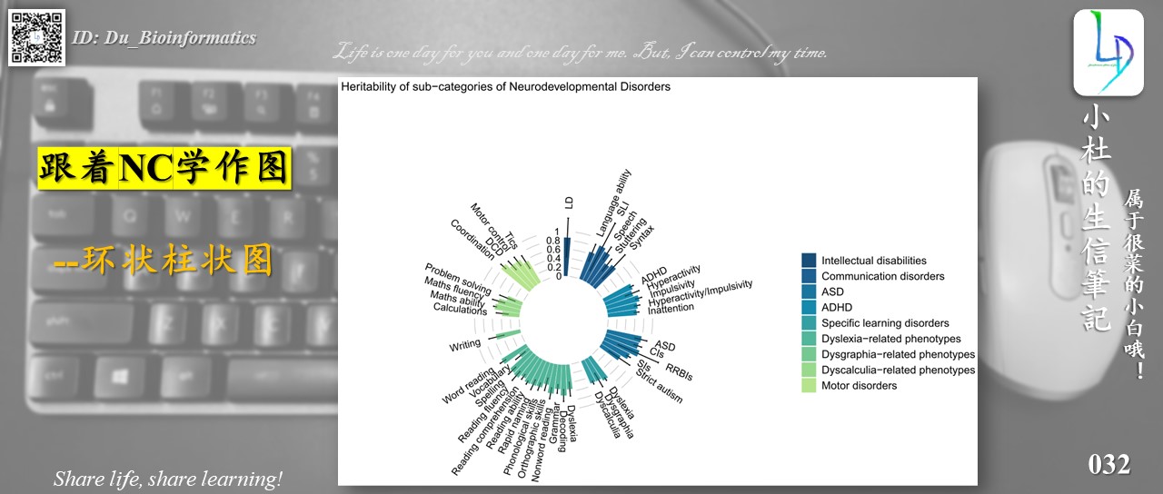
The graph drawn in this tutorial is from the NC journal. I don’t know what the graph is called, but if you look closely, it belongs to the “ringed histogram”, so that’s what it’s called!
It looks relatively new, so let’s learn it! !
Drawing
Load R package
library(ggplot2)
Load data

Draw basic graphics
p <- ggplot(data, aes(x=as.factor(id), y=est, fill=group)) + # Note that id is a factor. If x is numeric, there is some space between the first bar

  geom_bar(aes(x=as.factor(id), y=est, fill=group), stat="identity", alpha=1) +
  geom_errorbar(aes(ymin = est-se, ymax = est + se), width = 0.2, position = position_dodge(.9), size = .5, alpha=1)

Add a val
p2 <- p +
  geom_segment(data=grid_data, aes(x = end, y = 1, xend = start, yend = 1), color = "grey", alpha=1, size=0.3 , inherit.aes = FALSE ) +
  geom_segment(data=grid_data, aes(x = end, y = 0.8, xend = start, yend = 0.8), color = "grey", alpha=1, size=0.3 , inherit.aes = FALSE ) +
  geom_segment(data=grid_data, aes(x = end, y = 0.6, xend = start, yend = 0.6), color = "grey", alpha=1, size=0.3 , inherit.aes = FALSE ) +
  geom_segment(data=grid_data, aes(x = end, y = 0.4, xend = start, yend = 0.4), color = "grey", alpha=1, size=0.3 , inherit.aes = FALSE ) +
  geom_segment(data=grid_data, aes(x = end, y = 0.2, xend = start, yend = 0.2), color = "grey", alpha=1, size=0.3 , inherit.aes = FALSE ) +
  geom_segment(data=grid_data, aes(x = end, y = 0, xend = start, yend = 0), color = "grey", alpha=1, size=0.3 , inherit.aes = FALSE )

Add numbers to val
p3 <- p2 +
  annotate("text", x = rep(max(data$id),6), y = c(0, 0.2, 0.4, 0.6, 0.8, 1),
           label = c("0", "0.2", "0.4", "0.6", "0.8", "1") , color="black", size =4 , angle=0, hjust=1)

Extend the y-axis
p4 <- p3 +
  geom_bar(aes(x=as.factor(id), y=est, fill=group), stat="identity", alpha=0.5) +
  ylim(-1,3)

Beautify
p5 <- p4 +
  theme_minimal() +
  theme(
    legend.position = "right",
    legend.title = element_blank(),
    legend.text = element_text(size=12),
    axis.text = element_blank(),
    axis.title = element_blank(),
    panel. grid = element_blank())

Changes into a circular shape
Use the coord_polar() function to convert
p6 <- p5 + coord_polar()

Color beautification
p7 <- p6 + scale_fill_manual(breaks = c("Intellectual disabilities",
                                        "Communication disorders",
                                        "ASD",
                                        "ADHD",
                                        "Specific learning disorders",
                                        "Dyslexia-related phenotypes",
                                        "Dysgraphia-related phenotypes",
                                        "Dyscalculia-related phenotypes",
                                        "Motor disorders"),
                             values = c("#184e77","#1e6091","#1a759f",
                                        "#168aad","#34a0a4","#52b69a",
                                        "#76c893","#99d98c","#b5e48c")) +
  ggtitle("Heritability of sub-categories of Neurodevelopmental Disorders")

The label is mapped to the column
p8 <- p7 +
  geom_text(data=label_data, aes(x=id, y= est + se + 0.2, label=pheno, hjust=hjust),
            color="black", alpha=1, size=4, angle= label_data$angle, inherit.aes = FALSE )

Complete code
ggplot(data, aes(x=as.factor(id), y=est, fill=group)) + # Note that id is a factor. If x is numeric, there is some space between the first bar

  geom_bar(aes(x=as.factor(id), y=est, fill=group), stat="identity", alpha=1) +
  geom_errorbar(aes(ymin = est-se, ymax = est + se), width = 0.2, position = position_dodge(.9), size = .5, alpha=1) +

  # add val
  geom_segment(data=grid_data, aes(x = end, y = 1, xend = start, yend = 1), color = "grey", alpha=1, size=0.3 , inherit.aes = FALSE ) +
  geom_segment(data=grid_data, aes(x = end, y = 0.8, xend = start, yend = 0.8), color = "grey", alpha=1, size=0.3 , inherit.aes = FALSE ) +
  geom_segment(data=grid_data, aes(x = end, y = 0.6, xend = start, yend = 0.6), color = "grey", alpha=1, size=0.3 , inherit.aes = FALSE ) +
  geom_segment(data=grid_data, aes(x = end, y = 0.4, xend = start, yend = 0.4), color = "grey", alpha=1, size=0.3 , inherit.aes = FALSE ) +
  geom_segment(data=grid_data, aes(x = end, y = 0.2, xend = start, yend = 0.2), color = "grey", alpha=1, size=0.3 , inherit.aes = FALSE ) +
  geom_segment(data=grid_data, aes(x = end, y = 0, xend = start, yend = 0), color = "grey", alpha=1, size=0.3 , inherit.aes = FALSE ) +

  # add the numbers in val
  annotate("text", x = rep(max(data$id),6), y = c(0, 0.2, 0.4, 0.6, 0.8, 1),
           label = c("0", "0.2", "0.4", "0.6", "0.8", "1") , color="black", size =4 , angle=0, hjust=1) +

  geom_bar(aes(x=as.factor(id), y=est, fill=group), stat="identity", alpha=0.5) +
  ylim(-1,3) +
  theme_minimal() +
  theme(
    legend.position = "right",
    legend.title = element_blank(),
    legend.text = element_text(size=12),
    axis.text = element_blank(),
    axis.title = element_blank(),
    panel.grid = element_blank()) +
  ## change ring
  coord_polar() +
  ## Column annotation
  scale_fill_manual(breaks = c("Intellectual disabilities",
                               "Communication disorders",
                               "ASD",
                               "ADHD",
                               "Specific learning disorders",
                               "Dyslexia-related phenotypes",
                               "Dysgraphia-related phenotypes",
                               "Dyscalculia-related phenotypes",
                               "Motor disorders"),
                    ## column color
                    values = c("#184e77","#1e6091","#1a759f",
                               "#168aad","#34a0a4","#52b69a",
                               "#76c893","#99d98c","#b5e48c")) +
  ggtitle("Heritability of sub-categories of Neurodevelopmental Disorders") +
## Map labels to columns
  geom_text(data=label_data, aes(x=id, y= est + se + 0.2, label=pheno, hjust=hjust),
            color="black", alpha=1, size=4, angle= label_data$angle, inherit.aes = FALSE )
ENDING!
Previous articles:
1. The most complete WGCNA tutorial (replace the data to get all the results and graphics)
WGCNA Analysis | Whole Process Analysis Code | Code 1
WGCNA Analysis | Whole Process Analysis Code | Code 2
WGCNA Analysis | Whole Process Code Sharing | Code Three
2. Beautiful graphics drawing tutorial
Beautiful graphics drawing tutorial
It is said that the official account needs to be starred, so that you will not miss the content of the official account. So, let’s mark it too.


Xiao Du’s life letter notes, which mainly publish or include bioinformatics tutorials, as well as R-based analysis and visualization (including data analysis, graph drawing, etc.); share interested literature and learning materials!!