Welcome to follow the WeChat official account (Medical Bioinformatics), medical students’ student notes to record the learning process.
Common image formats include: pdf, jpeg, tiff, png, svg, wmf.
pdf, svg and wmf are vector graphics formats, so there will be no blur when enlarging the picture.
jpeg, tiff and png are bitmap formats and will appear blurry when resizing the file.
ggsave() to save images
If you draw through ggplot2, you can use ggsave() to save the output image.
plot1 <- ggplot(mtcars, aes(x = wt, y = mpg)) +
  geom_point()

#The default output unit is inches. The units can be specified through the units parameter.
ggsave("myplot.pdf", plot1, width = 8, height = 8, units = "cm")
Another way is to not assign the ggplot object to plot1, and only call ggsave() after calling ggplot() >, which will save the last ggplot object.
With ggsave(), there is no need to print the ggplot object through print(). If an error occurs when creating or saving the image, there is no need to pass print(). code>dev.off() to manually turn off the graphics device. Another thing to note is that ggsave() cannot be used to draw multi-page images.
ggplot(mtcars, aes(x = wt, y = mpg)) +
  geom_point()

ggsave("myplot.pdf", width = 8, height = 8, units = "cm")
Output pictures in PDF format
Method 1
pdf("myplot.pdf", width = 4, height = 4)

plot(mtcars$wt, mtcars$mpg)
print(ggplot(mtcars, aes(x = wt, y = mpg)) + geom_point())

dev.off()
The default output unit of width and height is inches. If you want to output the unit in centimeters, you need to convert it through the code below.
# 8x8 cm
pdf("myplot.pdf", width = 8/2.54, height = 8/2.54)
Method 2
plot1 <- ggplot(mtcars, aes(x = wt, y = mpg)) +
  geom_point()

#The default output unit is inches. The units can be specified through the units parameter.
ggsave("myplot.pdf", plot1, width = 8, height = 8, units = "cm")
Output images in SVG format
Method 1
library(svglite)
svglite("myplot.svg", width = 4, height = 4)
plot1 <- ggplot(mtcars, aes(x = wt, y = mpg)) +
  geom_point()
print(plot1)
dev.off()
Method 2
plot1 <- ggplot(mtcars, aes(x = wt, y = mpg)) +
  geom_point()
ggsave("myplot.svg", plot1, width = 8, height = 8, units = "cm")
Output images in PNG format
Method 1
# Width and height in pixels
png("myplot.png", width = 400, height = 400)
plot(mtcars$wt, mtcars$mpg)
dev.off()
To output multiple images, you can add %d to the file name.
png("myplot-%d.png", width = 400, height = 400)
plot(mtcars$wt, mtcars$mpg)
print(ggplot(mtcars, aes(x = wt, y = mpg)) + geom_point())
dev.off()
Default output is 72 pixels per inch (ppi). This resolution is suitable for display on electronic screens, while 300 ppi is generally used for printing.
ppi <- 300
# Calculate the height and width (in pixels) of a 4x4 inch image at 300 ppi
png("myplot.png", width = 4*ppi, height = 4*ppi, res = ppi)
plot(mtcars$wt, mtcars$mpg)
dev.off()

Method 2
ggplot(mtcars, aes(x = wt, y = mpg)) + geom_point()

#The default output unit is inches. The units can be specified through the units parameter.
ggsave("myplot.png", width = 8, height = 8, unit = "cm", dpi = 300)
Output pictures in TIFF format
Method 1
tiff("myplot.tiff", width = 4, height = 4, units = "cm", res = 300)
plot1 <- ggplot(mtcars, aes(x = wt, y = mpg)) +
  geom_point()
print(plot1)
dev.off()
Method 2
plot1 <- ggplot(mtcars, aes(x = wt, y = mpg)) +
  geom_point()
ggsave("myplot.tiff", plot1, width = 8, height = 8, units = "cm", dpi = 300)
Output pictures in WMF format
WMF files are created and used much like PDF files, but they can only be created on Windows.
Method 1
win.metafile("myplot.wmf", width = 4, height = 4)
plot1 <- ggplot(mtcars, aes(x = wt, y = mpg)) +
  geom_point()
print(plot1)
dev.off()
Method 2
plot1 <- ggplot(mtcars, aes(x = wt, y = mpg)) +
  geom_point()
ggsave("myplot.wmf", plot1, width = 8, height = 8, units = "cm")
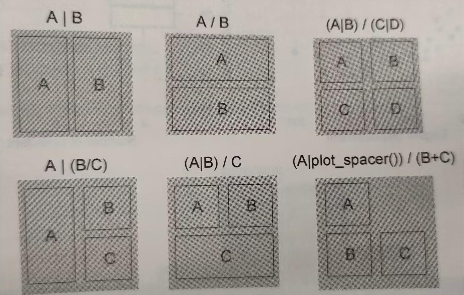
Puzzle
library(patchwork)
library(ggplot2)

plot1 <- ggplot(PlantGrowth, aes(x = weight)) +
  geom_histogram(bins = 12)

plot2 <- ggplot(PlantGrowth, aes(x = group, y = weight, group = group)) +
  geom_boxplot()

plot1 + plot2

library(patchwork)
library(ggplot2)
plot1 <- ggplot(PlantGrowth, aes(x = weight)) +
  geom_histogram(bins = 12)

plot2 <- ggplot(PlantGrowth, aes(x = group, y = weight, group = group)) +
  geom_boxplot()

plot3 <- ggplot(PlantGrowth, aes(x = weight, fill = group)) +
  geom_density(alpha = 0.25)

plot1 + plot2 + plot3 +
  plot_layout(ncol = 2)

library(patchwork)
library(ggplot2)
plot1 <- ggplot(PlantGrowth, aes(x = weight)) +
  geom_histogram(bins = 12)

plot2 <- ggplot(PlantGrowth, aes(x = group, y = weight, group = group)) +
  geom_boxplot()

plot3 <- ggplot(PlantGrowth, aes(x = weight, fill = group)) +
  geom_density(alpha = 0.25)

plot1 + plot2 +
  plot_layout(ncol = 1, heights = c(1, 4))

library(patchwork)
library(ggplot2)

p1 <- ggplot(mpg) +
  geom_point(aes(x = displ, y = hwy))

p2 <- ggplot(mpg) +
  geom_bar(aes(x = as.character(year), fill = drv), position = "dodge") +
  labs(x = "year")

p1/p2

library(patchwork)
library(ggplot2)

p3 <- ggplot(mpg) +
  geom_density(aes(x = hwy, fill = drv), color = NA) +
  facet_grid(rows = vars(drv))

p4 <- ggplot(mpg) +
  stat_summary(aes(x = drv, y = hwy, fill = drv), geom = "col", fun.data = mean_se) +
  stat_summary(aes(x = drv, y = hwy), geom = "errorbar", fun.data = mean_se, width = 0.5)

p3 | p4

library(patchwork)
library(ggplot2)

p1 <- ggplot(mpg) +
  geom_point(aes(x = displ, y = hwy))

p2 <- ggplot(mpg) +
  geom_bar(aes(x = as.character(year), fill = drv), position = "dodge") +
  labs(x = "year")

p3 <- ggplot(mpg) +
  geom_density(aes(x = hwy, fill = drv), color = NA) +
  facet_grid(rows = vars(drv))

p4 <- ggplot(mpg) +
  stat_summary(aes(x = drv, y = hwy, fill = drv), geom = "col", fun.data = mean_se) +
  stat_summary(aes(x = drv, y = hwy), geom = "errorbar", fun.data = mean_se, width = 0.5)

p3 | (p2 / (p1 | p4))

library(patchwork)
library(ggplot2)

p1 <- ggplot(mpg) +
  geom_point(aes(x = displ, y = hwy))

p2 <- ggplot(mpg) +
  geom_bar(aes(x = as.character(year), fill = drv), position = "dodge") +
  labs(x = "year")

p3 <- ggplot(mpg) +
  geom_density(aes(x = hwy, fill = drv), color = NA) +
  facet_grid(rows = vars(drv))

p4 <- ggplot(mpg) +
  stat_summary(aes(x = drv, y = hwy, fill = drv), geom = "col", fun.data = mean_se) +
  stat_summary(aes(x = drv, y = hwy), geom = "errorbar", fun.data = mean_se, width = 0.5)

layout <- "
AAB
C#B
CDD
"

p1 + p2 + p3 + p4 + plot_layout(design = layout)

library(patchwork)
library(ggplot2)

p1 <- ggplot(mpg) +
  geom_point(aes(x = displ, y = hwy))

p2 <- ggplot(mpg) +
  geom_bar(aes(x = as.character(year), fill = drv), position = "dodge") +
  labs(x = "year")

p3 <- ggplot(mpg) +
  geom_density(aes(x = hwy, fill = drv), color = NA) +
  facet_grid(rows = vars(drv))

p1 + p2 + p3 + plot_layout(ncol = 2, guides = "collect")

library(patchwork)
library(ggplot2)

p1 <- ggplot(mpg) +
  geom_point(aes(x = displ, y = hwy))

p2 <- ggplot(mpg) +
  geom_bar(aes(x = as.character(year), fill = drv), position = "dodge") +
  labs(x = "year")

p3 <- ggplot(mpg) +
  geom_density(aes(x = hwy, fill = drv), color = NA) +
  facet_grid(rows = vars(drv))

p1 + p2 + p3 + guide_area() + plot_layout(ncol = 2, guides = "collect")

library(patchwork)
library(ggplot2)

p1 <- ggplot(mpg) +
  geom_point(aes(x = displ, y = hwy))

p2 <- ggplot(mpg) +
  geom_bar(aes(x = as.character(year), fill = drv), position = "dodge") +
  labs(x = "year")

p12 <- p1 + p2
p12[[2]] <- p12[[2]] + theme_light()
p12

library(patchwork)
library(ggplot2)

p1 <- ggplot(mpg) +
  geom_point(aes(x = displ, y = hwy))

p4 <- ggplot(mpg) +
  stat_summary(aes(x = drv, y = hwy, fill = drv), geom = "col", fun.data = mean_se) +
  stat_summary(aes(x = drv, y = hwy), geom = "errorbar", fun.data = mean_se, width = 0.5)

p1 + p4 & theme_minimal()

library(patchwork)
library(ggplot2)

p1 <- ggplot(mpg) +
  geom_point(aes(x = displ, y = hwy))

p4 <- ggplot(mpg) +
  stat_summary(aes(x = drv, y = hwy, fill = drv), geom = "col", fun.data = mean_se) +
  stat_summary(aes(x = drv, y = hwy), geom = "errorbar", fun.data = mean_se, width = 0.5)

p1 + p4 & scale_y_continuous(limits = c(0, 45))

library(patchwork)
library(ggplot2)

p3 <- ggplot(mpg) +
  geom_density(aes(x = hwy, fill = drv), color = NA) +
  facet_grid(rows = vars(drv))

p4 <- ggplot(mpg) +
  stat_summary(aes(x = drv, y = hwy, fill = drv), geom = "col", fun.data = mean_se) +
  stat_summary(aes(x = drv, y = hwy), geom = "errorbar", fun.data = mean_se, width = 0.5)

p34 <- p3 + p4 + plot_annotation(
  title = "A closer look at the effect of drive train in cars",
  caption = "Source: mpg dataset in ggplot2"
)
p34

library(patchwork)
library(ggplot2)

p3 <- ggplot(mpg) +
  geom_density(aes(x = hwy, fill = drv), color = NA) +
  facet_grid(rows = vars(drv))

p4 <- ggplot(mpg) +
  stat_summary(aes(x = drv, y = hwy, fill = drv), geom = "col", fun.data = mean_se) +
  stat_summary(aes(x = drv, y = hwy), geom = "errorbar", fun.data = mean_se, width = 0.5)

p34 <- p3 + p4 + plot_annotation(
  title = "A closer look at the effect of drive train in cars",
  caption = "Source: mpg dataset in ggplot2"
)
p34 + plot_annotation(theme = theme_gray(base_family = "mono"))

library(patchwork)
library(ggplot2)

p3 <- ggplot(mpg) +
  geom_density(aes(x = hwy, fill = drv), color = NA) +
  facet_grid(rows = vars(drv))

p4 <- ggplot(mpg) +
  stat_summary(aes(x = drv, y = hwy, fill = drv), geom = "col", fun.data = mean_se) +
  stat_summary(aes(x = drv, y = hwy), geom = "errorbar", fun.data = mean_se, width = 0.5)

p34 <- p3 + p4 + plot_annotation(
  title = "A closer look at the effect of drive train in cars",
  caption = "Source: mpg dataset in ggplot2"
)
p34 & theme_gray(base_family = "mono")

library(patchwork)
library(ggplot2)

p1 <- ggplot(mpg) +
  geom_point(aes(x = displ, y = hwy))

p2 <- ggplot(mpg) +
  geom_bar(aes(x = as.character(year), fill = drv), position = "dodge") +
  labs(x = "year")

p3 <- ggplot(mpg) +
  geom_density(aes(x = hwy, fill = drv), color = NA) +
  facet_grid(rows = vars(drv))

p123 <- p1 | (p2 / p3)
p123 + plot_annotation(tag_levels = "I") # Uppercase roman numerics

library(patchwork)
library(ggplot2)

p1 <- ggplot(mpg) +
  geom_point(aes(x = displ, y = hwy))

p2 <- ggplot(mpg) +
  geom_bar(aes(x = as.character(year), fill = drv), position = "dodge") +
  labs(x = "year")

p3 <- ggplot(mpg) +
  geom_density(aes(x = hwy, fill = drv), color = NA) +
  facet_grid(rows = vars(drv))

p123 <- p1 | (p2 / p3)
p123[[2]] <- p123[[2]] + plot_layout(tag_level = "new")
p123 + plot_annotation(tag_levels = c("I", "a"))

library(patchwork)
library(ggplot2)

p1 <- ggplot(mpg) +
  geom_point(aes(x = displ, y = hwy))

p2 <- ggplot(mpg) +
  geom_bar(aes(x = as.character(year), fill = drv), position = "dodge") +
  labs(x = "year")

p1 + inset_element(p2, left = 0.5, bottom = 0.4, right = 0.9, top = 0.95)

The position is specified by given the left, right, top, and bottom location of the inset. The default is to use npc units which goes from 0 to 1 in the given area, but any grid::unit() can be used by giving them explicitly. The location is by default set to the panel area, but this can be changed with the align_to argument. Combining all this we can place an inset exactly 15 mm from the top right corner like this:
library(patchwork)
library(ggplot2)

p1 <- ggplot(mpg) +
  geom_point(aes(x = displ, y = hwy))

p2 <- ggplot(mpg) +
  geom_bar(aes(x = as.character(year), fill = drv), position = "dodge") +
  labs(x = "year")

p1+
  inset_element(
    p2,
    left = 0.4,
    bottom = 0.4,
    right = unit(1, "npc") - unit(15, "mm"),
    top = unit(1, "npc") - unit(15, "mm"),
    align_to = "full"
  )

library(patchwork)
library(ggplot2)

p1 <- ggplot(mpg) +
  geom_point(aes(x = displ, y = hwy))

p2 <- ggplot(mpg) +
  geom_bar(aes(x = as.character(year), fill = drv), position = "dodge") +
  labs(x = "year")

p4 <- ggplot(mpg) +
  stat_summary(aes(x = drv, y = hwy, fill = drv), geom = "col", fun.data = mean_se) +
  stat_summary(aes(x = drv, y = hwy), geom = "errorbar", fun.data = mean_se, width = 0.5)

p24 <- p2 / p4 + plot_layout(guides = "collect")
p1 + inset_element(p24, left = 0.5, bottom = 0.05, right = 0.95, top = 0.9)

library(patchwork)
library(ggplot2)

p1 <- ggplot(mpg) +
  geom_point(aes(x = displ, y = hwy))

p2 <- ggplot(mpg) +
  geom_bar(aes(x = as.character(year), fill = drv), position = "dodge") +
  labs(x = "year")

p12 <- p1 + inset_element(p2, left = 0.5, bottom = 0.5, right = 0.9, top = 0.95)
p12 & theme_bw()

library(patchwork)
library(ggplot2)

p1 <- ggplot(mpg) +
  geom_point(aes(x = displ, y = hwy))

p2 <- ggplot(mpg) +
  geom_bar(aes(x = as.character(year), fill = drv), position = "dodge") +
  labs(x = "year")

p12 <- p1 + inset_element(p2, left = 0.5, bottom = 0.5, right = 0.9, top = 0.95)
p12 + plot_annotation(tag_levels = "A")

For more details, please refer to: https://github.com/thomasp85/patchwork
useDingbatsparameters
When retouching in Adobe Illustrator, circles in the PDF may be drawn as font characters. This situation can be avoided by setting useDingbats = FALSE.
pdf("myplot.pdf", width = 4, height = 4, useDingbats = FALSE)

# or
ggsave("myplot.pdf", width = 4, height = 4, useDingbats = FALSE)
Reference materials
- R language practice (3rd edition)
- ggplot2: Data Analysis and Graphic Arts (2nd Edition)
- R language medical data analysis practice
- https://ggplot2-book.org/arranging-plots
- https://r-graphics.org/