Hello everyone, I am taking me to ski!
For unknown nonlinear functions, it is difficult to find the extreme value of the function only through the input and output data of the function. This type of problem can be solved through neural networks combined with genetic algorithms, using the nonlinear fitting capabilities of neural networks and the nonlinear search of genetic algorithms. Excellent ability to find extreme values of functions.
Table of Contents
1. Problems and models
(1) Solve the problem
(2) Model building ideas
2. Code implementation
(1) BP neural network training
(3) Fitness function
(4) Genetic algorithm main function
1. Problems and models
(1) Solve the problem
Use the neural network genetic algorithm to find the extreme value of the nonlinear function. The expression of the function is:

The graph of the function is:
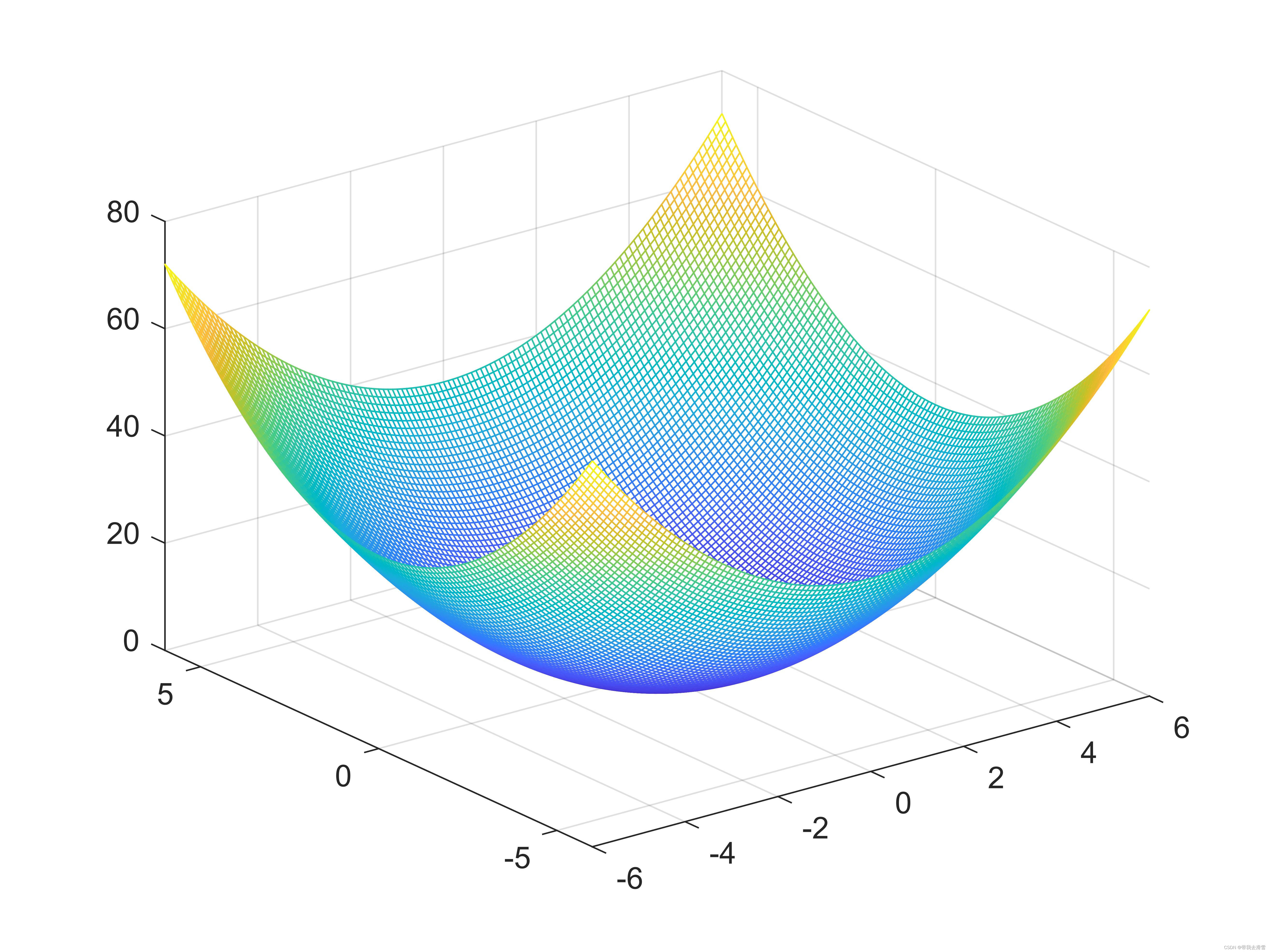
Through the function image, it can be seen more intuitively that the global minimum value of the function is 0, and the corresponding coordinates are (0, 0). Although it is easy to find the function extreme value and its corresponding coordinates from functional equations and graphs, it is difficult to find the function extreme value and its corresponding coordinates when the function equation is unknown.
(2) Model building ideas
Neural network training and fitting constructs a suitable BP neural network based on the characteristics of the optimization function, and uses the input and output data of the nonlinear function to train the BP neural network. The trained BP neural network can predict the function output. Genetic algorithm extreme value optimization uses the trained BP neural network prediction results as individual fitness values, and finds the global optimal value of the function and the corresponding input value through selection, crossover, and mutation operations.
Determine the model structure of the BP neural network to be 2-5-1, take 4000 sets of input and output data of the function, randomly select 3500 sets of data to train the neural network, and 100 sets of data to test the performance of the neural network. After the network is trained, it is used to predict nonlinearity function output.
In the genetic algorithm, individuals are encoded with real numbers. Since the optimization function has only two input parameters, the individual length is 2. The individual fitness value is the predicted value of BP neural network. The smaller the fitness value, the better the individual. Set the crossover probability to 0.4 and the mutation probability to 0.2.
2. Code implementation
(1) BP neural network training
clc
clear
tic
load data1 input output
k=rand(1,4000);
[m,n]=sort(k);
input_train=input(n(1:3900),:)';
output_train=output(n(1:3900),:)';
input_test=input(n(3901:4000),:)';
output_test=output(n(3901:4000),:)';
[inputn,inputps]=mapminmax(input_train);
[outputn,outputps]=mapminmax(output_train);
net=newff(inputn,outputn,5);
net.trainParam.epochs=100;
net.trainParam.lr=0.1;
net.trainParam.goal=0.0000004;
net=train(net,inputn,outputn);
inputn_test=mapminmax('apply',input_test,inputps);
an=sim(net,inputn_test);
BPoutput=mapminmax('reverse',an,outputps);
figure(1)
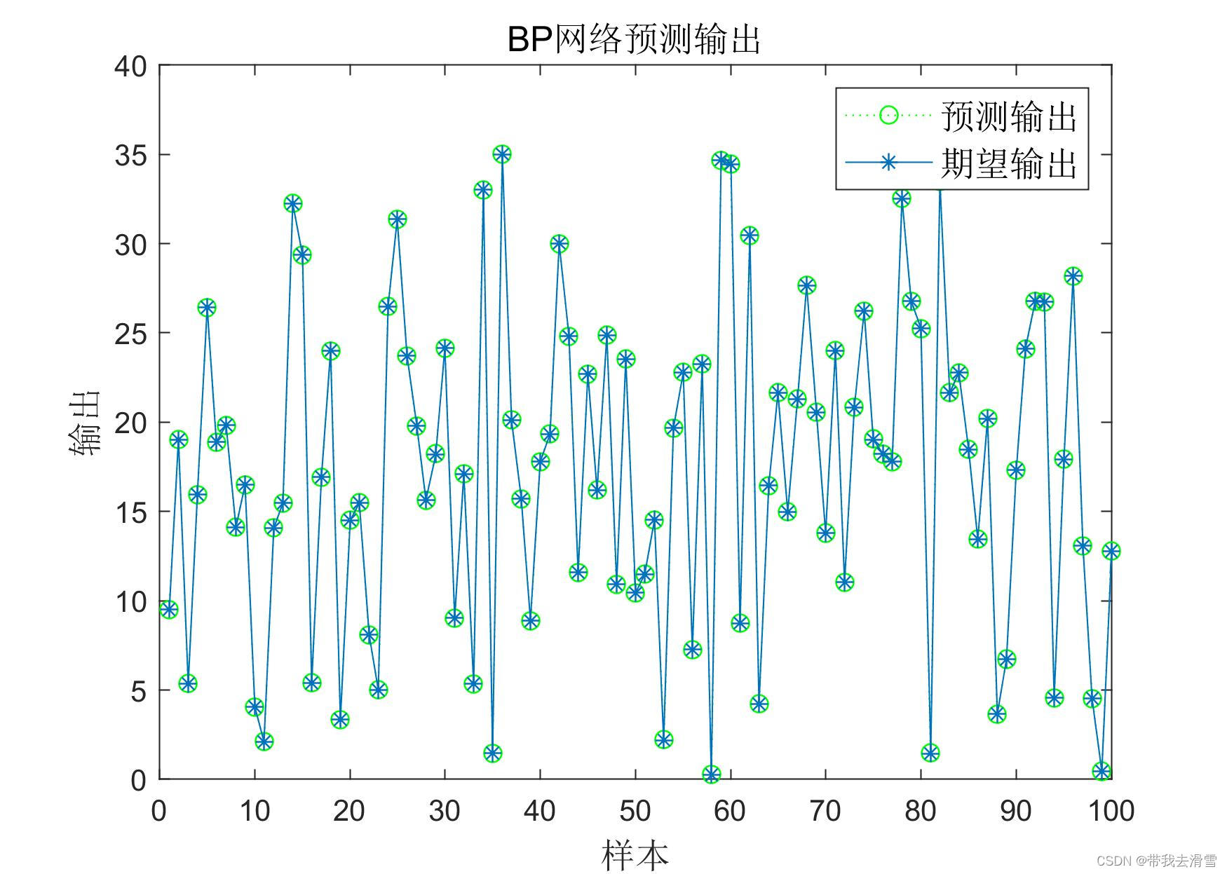
plot(BPoutput,':og')
hold on
plot(output_test,'-*');
legend('predicted output','expected output','fontsize',12)
title('BP network prediction output','fontsize',12)
xlabel('sample','fontsize',12)
ylabel('output','fontsize',12)
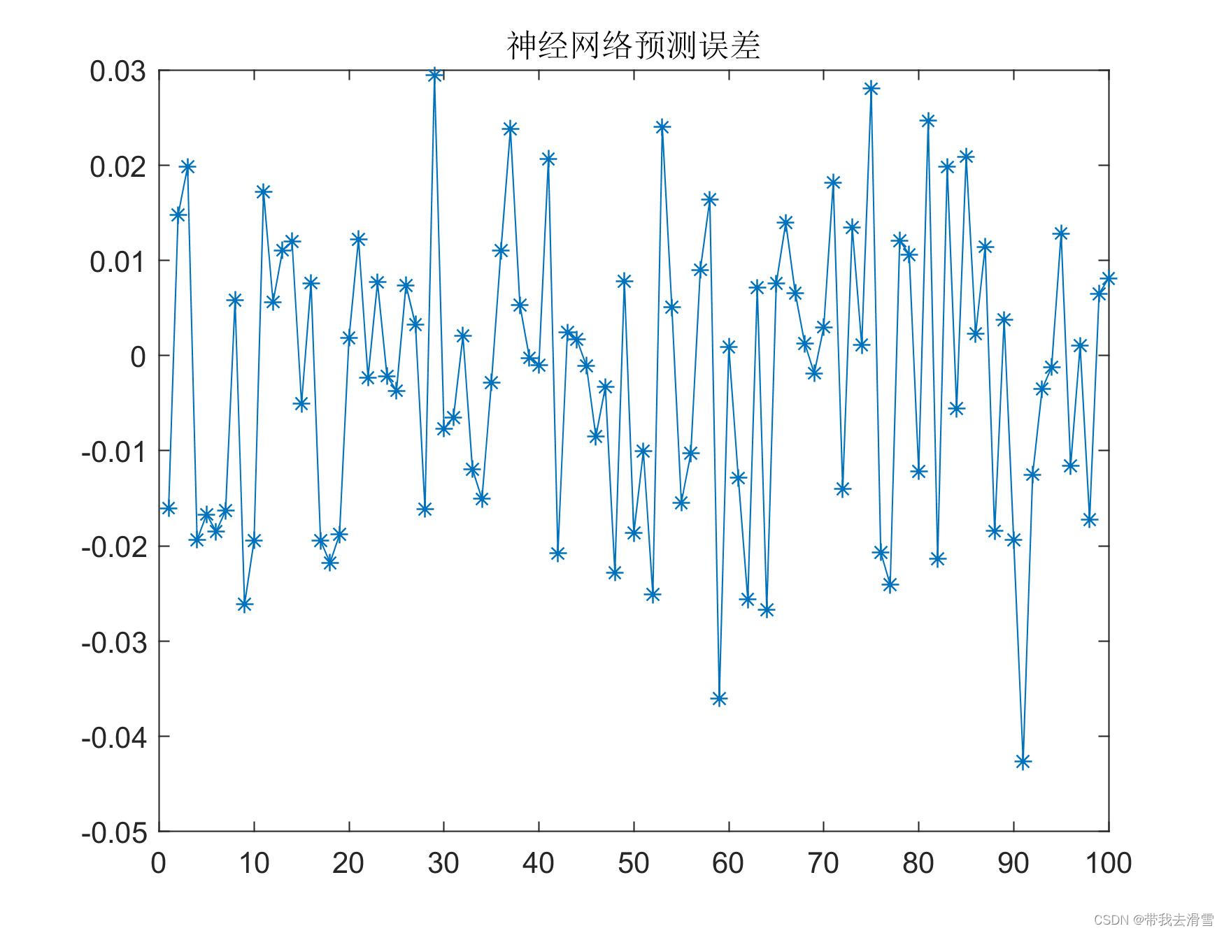
error=BPoutput-output_test;
figure(2)
plot(error,'-*')
title('Neural network prediction error')
figure(3)
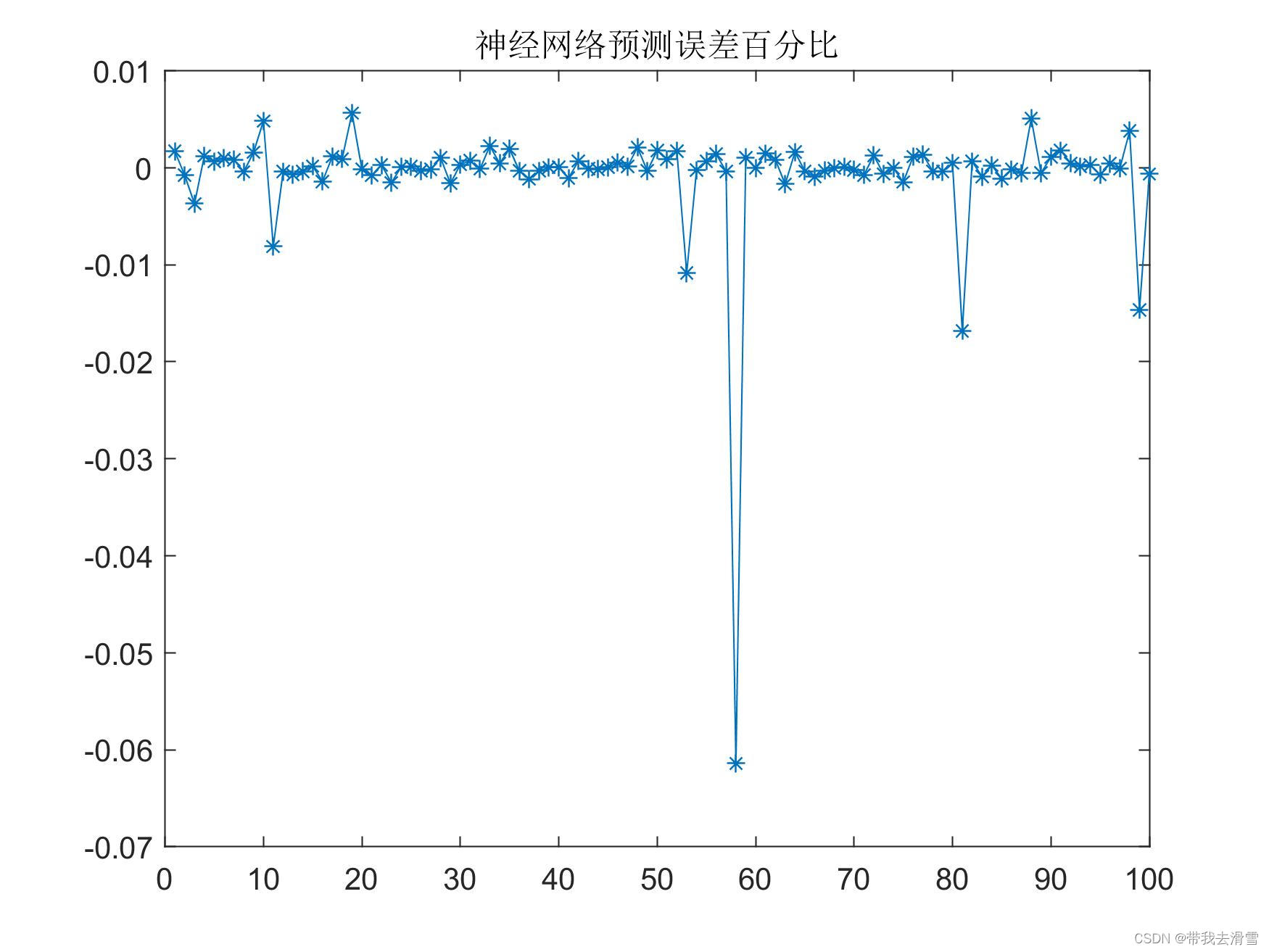
plot((output_test-BPoutput)./BPoutput,'-*');
title('Neural network prediction error percentage')
errorsum=sum(abs(error))
toc
save data net inputps outputps
Output result:
BP neural network prediction error percentage chart:
BP neural network prediction error graph:
BP neural network prediction result chart:
Validation set mean square error iteration plot:
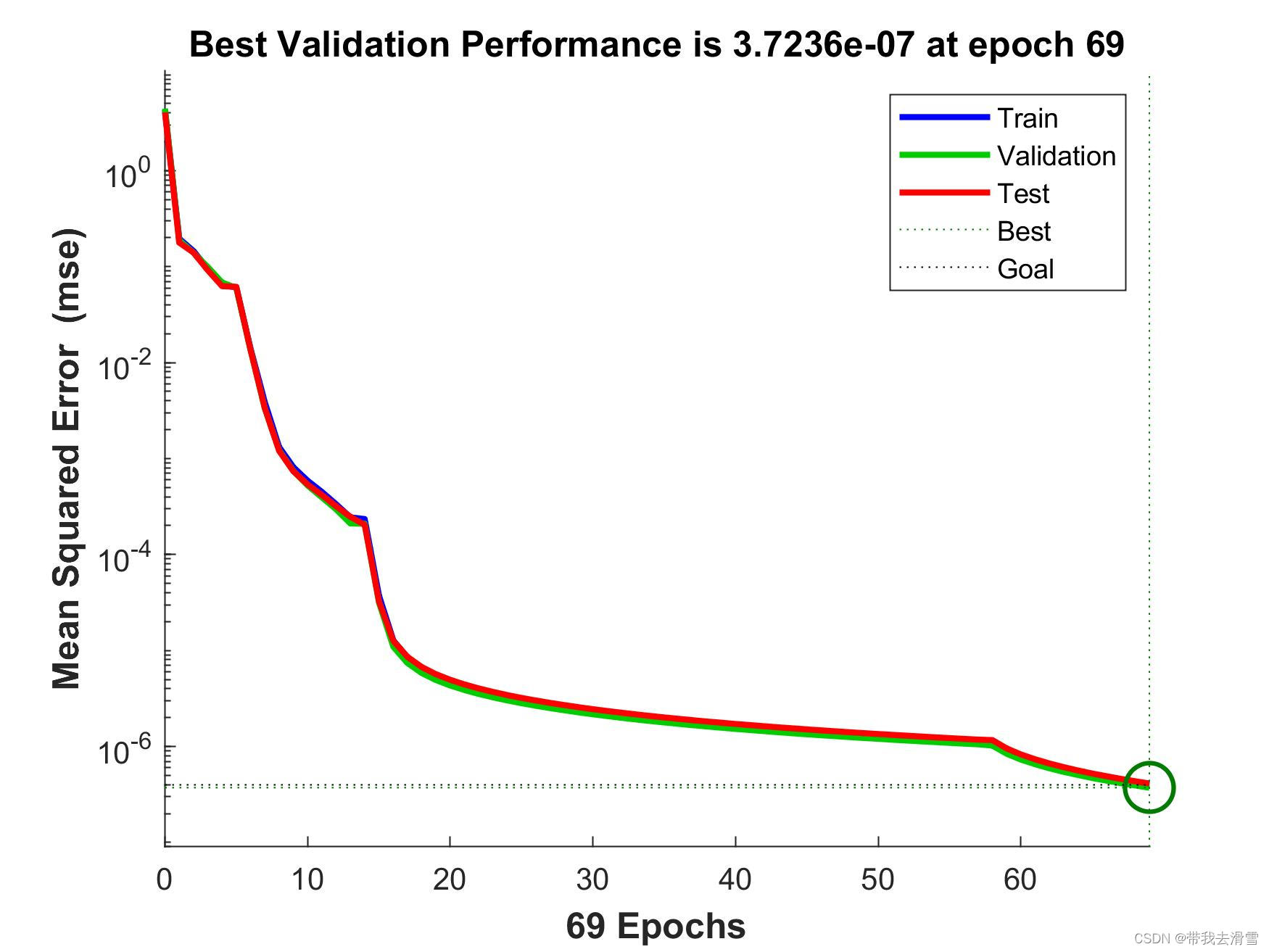
(3) Fitness function
Use the trained BP neural network prediction output as the individual fitness value:
function fitness = fun(x)
load data net inputps outputps
x=x';
inputn_test=mapminmax('apply',x,inputps);

an=sim(net,inputn_test);
fitness=mapminmax('reverse',an,outputps);
(4) Genetic algorithm main function
clc
clear

%% Initialize genetic algorithm parameters
%Initialization parameters
maxgen=100; %evolutionary algebra, that is, the number of iterations
sizepop=20; %population size
pcross=[0.4]; %cross probability selection, between 0 and 1
pmutation=[0.2]; % mutation probability selection, between 0 and 1

lenchrom=[1 1]; %The string length of each variable. If it is a floating point variable, the length is 1
bound=[-5 5;-5 5]; % data range


individuals=struct('fitness',zeros(1,sizepop), 'chrom',[]); %define population information as a structure
avgfitness=[]; % average fitness of each generation population
bestfitness=[]; %The best fitness of each generation population
bestchrom=[]; %The chromosome with the best fitness

%% Initialize the population to calculate fitness value
% initialize population
for i=1:sizepop
    % Randomly generate a population
    individuals.chrom(i,:)=Code(lenchrom,bound);
    x=individuals.chrom(i,:);
    % Calculate fitness
    individuals.fitness(i)=fun(x); % chromosome fitness
end
%Find the best chromosome
[bestfitness bestindex]=min(individuals.fitness);
bestchrom=individuals.chrom(bestindex,:); %The best chromosome
avgfitness=sum(individuals.fitness)/sizepop; %average fitness of chromosomes
% Record the best fitness and average fitness in each generation of evolution
trace=[avgfitness bestfitness];

%% Iterative optimization
% Evolution begins
for i=1:maxgen
    i
    % choose
    individuals=Select(individuals,sizepop);
    avgfitness=sum(individuals.fitness)/sizepop;
    %cross
    individuals.chrom=Cross(pcross,lenchrom,individuals.chrom,sizepop,bound);
    % Mutations
    individuals.chrom=Mutation(pmutation,lenchrom,individuals.chrom,sizepop,[i maxgen],bound);

    % Calculate fitness
    for j=1:sizepop
        individuals.fitness(j)=fun(x);
    end

  %Find the chromosomes with minimum and maximum fitness and their positions in the population
    [newbestfitness,newbestindex]=min(individuals.fitness);
    [worestfitness,worestindex]=max(individuals.fitness);
    % replaces the best chromosome from the last evolution
    if bestfitness>newbestfitness
        bestfitness=newbestfitness;
        bestchrom=individuals.chrom(newbestindex,:);
    end
    individuals.chrom(worestindex,:)=bestchrom;
    individuals.fitness(worestindex)=bestfitness;


    trace=[trace;avgfitness bestfitness]; %Record the best fitness and average fitness in each generation of evolution
end
%Evolution ends

%% Result analysis
[r c]=size(trace);
plot([1:r]',trace(:,2),'r-');
title('Fitness Curve','fontsize',12);
xlabel('Evolutionary algebra','fontsize',12);ylabel('Fitness','fontsize',12);
Output result:
The optimal individual fitness value change curve during the optimization process:
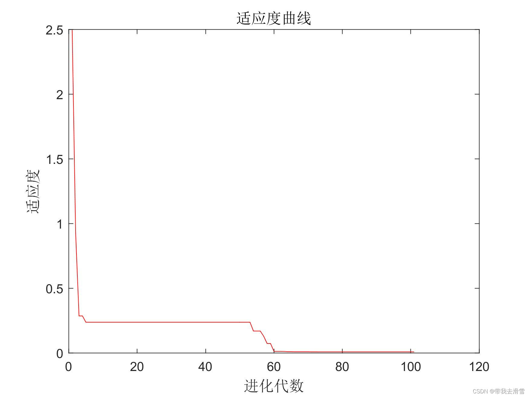
The optimal individual fitness value obtained by the genetic algorithm is 0.01, and the optimal individual is (-0.0081, 0.0014).
More high-quality content is being released continuously, please go to the homepage to view.
If you have any questions, please contact us via email: [email protected]
Blogger’s WeChat:TCB1736732074
Like + follow to avoid getting lost next time!
The knowledge points of the article match the official knowledge files, and you can further learn related knowledge. Algorithm skill tree Home page Overview 57455 people are learning the system