Topic 1: Gaussian noise with a mean value of 0 and a variance of 0.03 is added to 20 noisy images. Please denoise and enhance the images and write down the principle.

1. Algorithm principle:
Gaussian filtering is a linear smoothing filter, which is suitable for eliminating Gaussian noise and is widely used in the noise reduction process of image processing.
?In layman’s terms, Gaussian filtering is a process of weighted averaging of the entire image. The value of each pixel is obtained by weighted averaging of itself and other pixel values in the neighborhood.
The specific operation of Gaussian filtering is: use a template (or convolution, mask) to scan each pixel in the image, and use the weighted average gray value of the pixels in the neighborhood determined by the template to replace the value of the pixel in the center of the template.
? Corresponding to mean filtering and box filtering, the weight of each pixel in its neighborhood is equal. In Gaussian filtering, the weight value of the center point will be increased, and the weight value far away from the center point will be reduced. On this basis, the sum of different weights of each pixel value in the neighborhood is calculated.
20 noisy images:
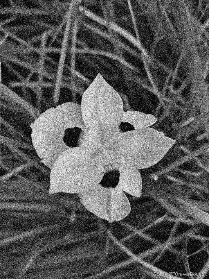
We averaged 20 noisy images using Gaussian filtering.
import numpy as np
import cv2

def GaussianFilter(img):
   h, w, c = img. shape
   print(img. shape)
   # Gaussian filter
   K_size = 3
   sigma = 1.3

   # zero padding
   pad = K_size // 2
   out = np. zeros((h + 2 * pad, w + 2 * pad, c), dtype=np. float)
   out[pad:pad + h, pad:pad + w] = img.astype(np.float)

   # define filter kernel
   K = np.zeros((K_size, K_size), dtype=np.float)

   for x in range(-pad, -pad + K_size):
       for y in range(-pad, -pad + K_size):
           K[y + pad, x + pad] = np.exp(-(x ** 2 + y ** 2) / (2 * (sigma ** 2)))
   K /= (sigma * np. sqrt(2 * np. pi))
   K /= K.sum() # Normalization

   # The process of convolution
   tmp = out. copy()
   for y in range(h):
       for x in range(w):
           for ci in range(c):
               out[pad + y, pad + x, ci] = np. sum(K * tmp[y:y + K_size, x:x + K_size, ci])

   out = out[pad:pad + h, pad:pad + w].astype(np.uint8)

   return out


if __name__ == "__main__":

   img_final = np. zeros((960, 720, 3), dtype=np. float)
   for i in range(20):
       img_name = "image_noise{i}.jpg".format(i=i + 1)
       img1 = cv2.imread(img_name)
       img2 = GaussianFilter(img1)
       img2 = img2.astype(np.float)
       img_final += img2
   img_final /= 20
   img_final = img_final.astype(np.uint8)
   cv2.imwrite("image_final.jpg", img_final)
Output result image_final.jpg:
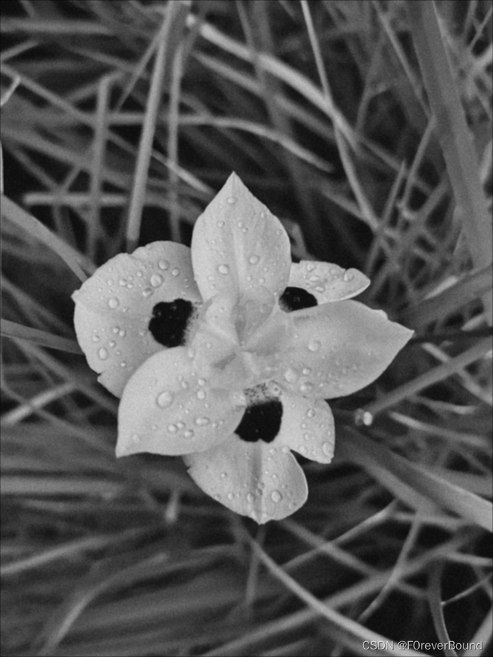
It can be seen that after Gaussian filtering and averaging of 20 noisy images, the obtained images are basically free of noise, clearer, and the quality has improved a lot.
Question 2: Please do a simple spatial mean filter on the following figure, the template is a 15*15 matrix, and use three different methods to consider the effect of boundary filtering.

1. Algorithm principle:
Mean filtering:
The output of a smooth linear spatial filter is a simple average of the pixels contained in the neighborhood of the filter template, that is, the mean filter. The average filter is also a low-pass filter, and the average filter is easy to understand, that is, the average value in the neighborhood is assigned to the center element.
The mean filter is used to reduce noise. The main application of the mean filter is to remove irrelevant details in the image. The irrelevance refers to the smaller pixel area compared with the template of the filter. Blurs the image to get a rough depiction of the object of interest, so that the grayscale of those smaller objects blends in with the background, and larger objects become blob-like and easier to detect. The size of the template is determined by the size of the objects that will be blended into the background.
The disadvantage of the mean filter is that there is a problem of blurred edges.
Boundary filtering is a basic image processing method in the field of digital image processing. It is mainly used to remove artifacts or noise at the edge of the image, and is often used in the pre-processing of image enhancement and feature extraction. The following are three different boundary filtering methods:
1. Reflective Boundary Filtering (Reflective Boundary Filtering): Reflective boundary filtering refers to using the mirror value of the boundary pixel as part of the convolution kernel during filtering. The advantage of this method is that the smoothness of the boundary is preserved and no additional noise is introduced.
2. Extended Boundary Filtering (Extended Boundary Filtering): Extended Boundary Filtering refers to extending the area outside the boundary by a certain pixel value during filtering. The advantage of this method is that it can effectively avoid boundary artifacts in the filtering results, but it will introduce additional noise at the edge of the image.
3. Zero Boundary Filtering: Zero Boundary Filtering refers to using the zero value of the boundary pixel value as part of the convolution kernel during filtering. This approach removes boundary artifacts, but filtering may result in image regions outside the smooth boundary relative to reflective boundary filtering.
import cv2
import numpy as np


def process(name, key):
   # read image
   img = cv2.imread(name)
   img = cv2.cvtColor(img, cv2.COLOR_BGR2GRAY)
   height, width = img. shape[:2]
   # Define filter template size
   kernel_size = 15

   if key == 'ZeroPadding':
       # define zero boundary filtering
       border_type = cv2.BORDER_CONSTANT
       border_value = 0
       # extend bounds
       img_expanded = cv2.copyMakeBorder(img, kernel_size // 2, kernel_size // 2, kernel_size // 2, kernel_size // 2,
                                         border_type, value=border_value)
   if key == 'Reflect':
       # define reflective boundary filter
       border_type = cv2.BORDER_REFLECT

       # reflective boundary filtering
       img_expanded = cv2.copyMakeBorder(img, kernel_size // 2, kernel_size // 2, kernel_size // 2, kernel_size // 2,
                                         border_type)
   if key == 'Replicate':
       # define extended boundary filter
       border_type = cv2.BORDER_REPLICATE
       # extend bounds
       img_expanded = cv2.copyMakeBorder(img, kernel_size // 2, kernel_size // 2, kernel_size // 2, kernel_size // 2,
                                         border_type)

   # mean filtering
   kernel = np.ones((kernel_size, kernel_size), np.float32) / (kernel_size ** 2)
   img_filtered = cv2. filter2D(img_expanded, -1, kernel)

   # Intercept the valid part
   img_filtered = img_filtered[kernel_size // 2: height + kernel_size // 2, kernel_size // 2: width + kernel_size // 2]

   # Show results
   cv2.imshow('Original', img)
   cv2.imshow(key, img_filtered)

if __name__ == "__main__":
   process("2.bmp", 'ZeroPadding')
   process("2.bmp", 'Reflect')
   process("2.bmp", 'Replicate')
   cv2.waitKey(0)
   cv2.destroyAllWindows()
Result graph:


The effects of the three methods to deal with boundary filtering are different.
Zero Boundary Filtering
In this method, the border area is filled with 0. This method can produce some noticeable black edges when dealing with edge parts.
Reflective Boundary Filtering
In this method, the image edges are inverted and duplicated to create a new pixel outside the edge image. Thus, a small area of pixels around the edge is reflective, and the effect of inverting the image is to create a “corner” of pixels (ie, a cell of pixels with no color information) around the edge.
Extended Boundary Filtering
In this method, pixel values are repeated on the border. This means that when an edge is reached, a small area around the edge will be stenciled using the values of the edge pixels. This results in repeated rows or columns in the image around the edges.
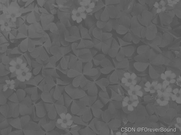
Question 3: Please use histogram equalization to enhance the following image.
Histogram equalization is a common image enhancement method, which can transform the histogram of the image to make the gray level distribution of the image more uniform, thereby enhancing the contrast and display effect of the image.
Histogram equalization is divided into the following steps:
First calculate the histogram of the original image, i.e. the number of pixels in each gray level in the image.
Calculate the cumulative distribution function (Cumulative Distribution Function, CDF) of the original image to obtain the probability of occurrence of each gray level in the entire image.
Scale the CDF to the maximum gray level (that is, image depth), and calculate a new mapping table, which maps the gray level value in the original image to the gray level after histogram equalization.
Use this new map to convert the gray level of each pixel in the original image to a new gray level and create a histogram-equalized image.
Through this process, histogram equalization can expand the dynamic range of the image, reduce the variance of pixel intensity values in the image, and enhance the contrast of the image, thereby improving the visual quality of the image.
import cv2
import numpy as np
def Origin_histogram(img):
   # Create a correspondence table between the gray value and the number of pixels of each gray level of the original image
   histogram = {}
   for i in range(img. shape[0]):
       for j in range(img. shape[1]):
           k = img[i][j]
           if k in histogram:
               histogram[k] + = 1
           else:
               histogram[k] = 1

   sorted_histogram = {} # Create a sorted mapping table
   sorted_list = sorted(histogram) # Sort from low to high according to the gray value

   for j in range(len(sorted_list)):
       sorted_histogram[sorted_list[j]] = histogram[sorted_list[j]]

   return sorted_histogram


def equalization_histogram(histogram, img):
   pr = {} # Create a probability distribution mapping table

   for i in histogram.keys():
       pr[i] = histogram[i] / (img.shape[0] * img.shape[1])

   tmp = 0
   for m in pr.keys():
       tmp + = pr[m]
       pr[m] = max(histogram) * tmp

   new_img = np.zeros(shape=(img.shape[0], img.shape[1]), dtype=np.uint8)

   for k in range(img. shape[0]):
       for l in range(img. shape[1]):
           new_img[k][l] = pr[img[k][l]]

   return new_img


if __name__ == '__main__':


# read raw image

img = cv2.imread('body_x_ray.jpg', cv2.IMREAD_GRAYSCALE)
# Calculate the original image grayscale histogram
origin_histogram = origin_histogram(img)

# Histogram equalization
new_img1 = equalization_histogram(origin_histogram, img)# perform histogram equalization


# Display the original image and the histogram-equalized image
cv2.imshow('original', img)
cv2.imshow('processed', new_img1)
cv2.waitKey(0) # wait for the user to press any key
result:

After obtaining the image after the equalization of the gray histogram, it can be seen that the leaves are “shine” a lot, the image becomes very clear, the texture of the leaves also appears, and the image quality is no longer gray.
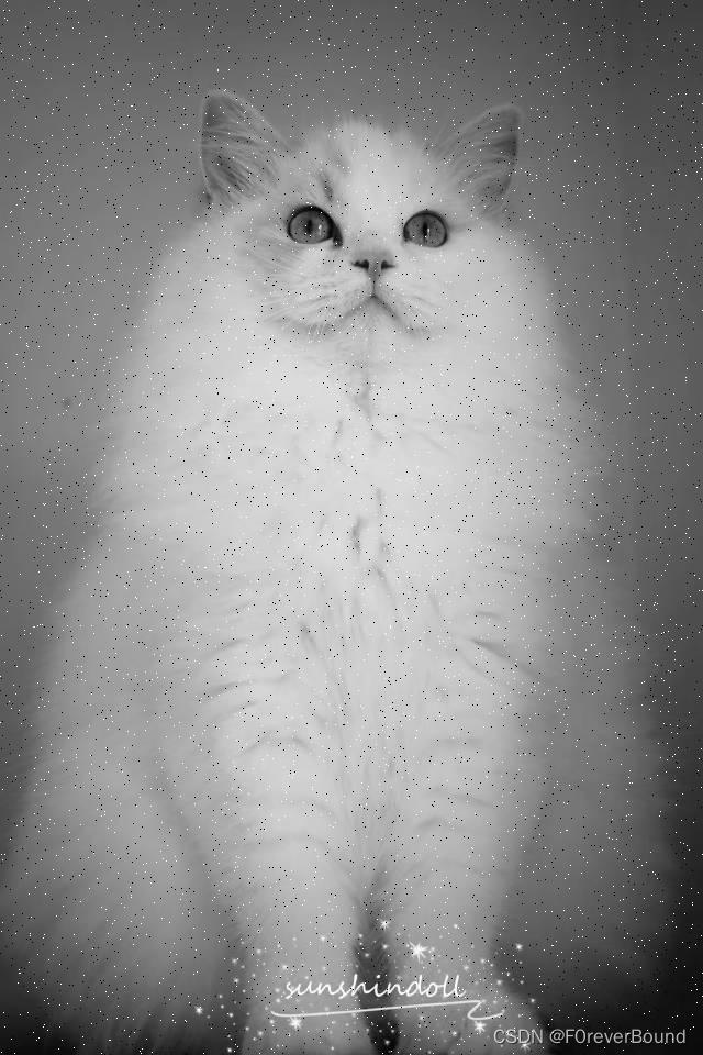
Question 4: Please do a gamma transformation on the image below to enhance its contrast.

Gamma transformation is a non-linear image enhancement method, which is mainly used to adjust the brightness, contrast and color balance of the image. Gamma transformation is to adjust the contrast and brightness of the image by adjusting the gamma value.
The main functions of gamma transformation include:
Improve contrast: For some images with low grayscale values, their contrast is very low, and it is difficult to show the details inside the image. By setting the gamma value to a value lower than 1, the brightness value of pixels with lower gray values in the image can be increased, which can improve the overall contrast of the image, thereby enhancing the visibility of the image.
Adjust brightness and color balance: In image processing, it is often necessary to adjust the brightness and color in the image. For images that are too dark, you can adjust the brightness by setting the gamma value to a value greater than 1. If the color distribution of the image is distorted or too washed out, it can be used for color balancing with a value larger than the given gamma value.
Application in image coding: Gamma transform is widely used in image coding. It can effectively eliminate a large amount of redundant information in image data and reduce the data size of images while maintaining image quality.
Gamma transformation is a practical image processing method. It can be used to improve image quality, adjust image brightness and color balance, etc., and enhance image visibility and practicability. It has a wide range of applications in image processing and computer vision. application value.
import cv2
import numpy as np
import matplotlib.pyplot as plt

# Read the image that needs to be processed
img = cv2.imread('1.jpg', cv2.IMREAD_GRAYSCALE)

# Set the gamma value
gamma = 0.5

# Perform gamma transformation on the image
gamma_correction = np.power(img / 255.0, gamma)
gamma_correction = (gamma_correction * 255).astype(np.uint8)

# Display the original image and the gamma-transformed image
fig = plt.figure(figsize=(10, 10))

ax1 = fig.add_subplot(2, 1, 1)
ax1.imshow(img, cmap='gray')
ax1. title. set_text("original")

ax2 = fig.add_subplot(2, 1, 2)
ax2.imshow(gamma_correction, cmap='gray')
ax2. title. set_text("processed")

plt. show()
result:

It can be seen that after the gamma transformation of the image, the brightness value of the pixel with a lower gray value in the image is increased, the overall contrast of the image is improved, and the visibility of the image is greatly enhanced.
Topic 5: Please use the mean filter and median filter to filter the image respectively, and analyze the processed results.
Median filtering:
Median filtering is a nonlinear signal processing method, so it is a nonlinear filter and a statistical sorting filter. It sets the gray value of each pixel as the median value of the gray values of all pixels in a certain neighborhood window of the point.
Median filtering has a good filtering effect on isolated noise pixels, namely salt and pepper noise and impulse noise, and can maintain the edge characteristics of the image without causing significant blurring of the image.
Median filtering is to replace the value of a point in a digital image or digital sequence with the median value of each point in a neighborhood of the point, so that the surrounding pixel values are close to the real value, thereby eliminating isolated noise points.
Mean filtering:
The output of a smooth linear spatial filter is a simple average of the pixels contained in the neighborhood of the filter template, that is, the mean filter. The average filter is also a low-pass filter, and the average filter is easy to understand, that is, the average value in the neighborhood is assigned to the center element.
The mean filter is used to reduce noise. The main application of the mean filter is to remove irrelevant details in the image. The irrelevance refers to the smaller pixel area compared with the template of the filter. Blurs the image to get a rough depiction of the object of interest, so that the grayscale of those smaller objects blends in with the background, and larger objects become blob-like and easier to detect. The size of the template is determined by the size of the objects that will be blended into the background.
The disadvantage of the mean filter is that there is a problem of blurred edges.
import cv2
import numpy as np


def MedianFilter(img, k=3):
   h, w = img. shape
   pad = k // 2
   out = np.zeros((h + 2 * pad, w + 2 * pad), dtype="uint8")
   out[pad:pad + h, pad:pad + w] = img.astype(np.float)
   for y in range(h):
       for x in range(w):
           out[pad + y, pad + x] = np.median(img[y:y + k, x:x + k]) # call np.median to find the median
   return out


def MeanFilter(img, k=3):
   h, w = img. shape
   pad = k // 2
   out = np.zeros((h + 2 * pad, w + 2 * pad), dtype="uint8")
   out[pad:pad + h, pad:pad + w] = img.astype(np.float)
   for y in range(h):
       for x in range(w):
           out[pad + y, pad + x] = np.mean(img[y:y + k, x:x + k]) # call np.mean to find the mean
   return out


if __name__ == "__main__":
   # process("image_salt_pepper2.jpg")
   img = cv2.imread("image_salt_pepper2.jpg", 0)
   result1 = MedianFilter(img)
   result2 = MeanFilter(img)
   cv2.imshow("Original", img)
   cv2.imshow("MedianFilter", result1)
   cv2.imshow("MeanFilter", result2)

   cv2.waitKey(0)
   cv2.destroyAllWindows()
Result graph:
Median filtering:

Mean filtering:

It can be seen that the median filter basically removes the noise of the image, and the mean filter still contains a small amount of noise, but the influence of the noise is weakened on average.
Both have the function of smoothing the image and filtering out the noise.