Optimization-Fibonacci Sequence (fibonacci) Optimization Method Algorithm Principle and Code Implementation

1. Model introduction

The Fibonacci sequence is also called the rabbit sequence. Its values are: 1, 1, 2, 3, 5, 8, 13, 21, 34… Mathematically, this sequence is defined by the following recursive method:

F(0)=1, F(1)=1, F(n)=F(n – 1) + F(n – 2) (n ≥ 2, n ∈ N*).

This article introduces the fibonacci sequence into the optimal one-dimensional search to solve the optimization.

2. Model principle

Advantages of the 2.1 model

The Fibonacci sequence is used in one-dimensional exploration of unimodal functions to find the optimal value. Its main advantage is that it solves two function values in the first iteration and only needs to solve it once in each subsequent iteration. Model definition:

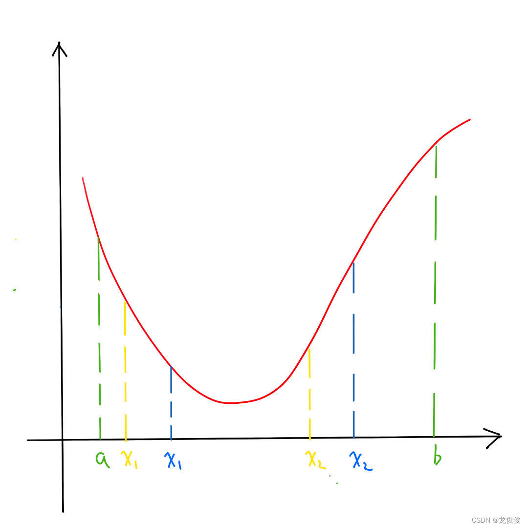
As shown in the figure: given initial value according to the model definition $a_k,b_k$ inferred:

$\lambda_k = a_k + \frac{f_n-k-1}{f_n-k + 1}*(b_k-a_k)$

$\mu_k = a_k + \frac{f_n-k}{f_n-k + 1}*(b_k-a_k)$

(1).When $f(\lambda_k)<f(\mu_k)$ : $a_{k + 1} = a_k ,b_{k + 1} = \mu_k$

(2).When $f(\lambda_k) \geq f(\mu_k):a_{k + 1}=\lambda_k,b_{k + 1} = b_k$ :

When the first condition is met, bringing in the simplification leads to:

$\mu_{k + 1} = \lambda_k$ , we only need to output $\lambda_{k + 1}$ That’s it

When the second condition is met, bringing in the simplification leads to:

$\lambda_{k + 1} = \mu_k$ , we only need to output $\mu_{k + 1}$ That’s it.

2.2 Algorithm design steps

(1) Given the initial interval $[a_n,b_n]$ , and the final interval length (accuracy) epsilon, find the number of times n to calculate the function value, so that

$F_n\geqslant (b_n-a_n)/epsilon$

Then calculate the trial point $x_1,x_2$

$x_1 = a_k + \frac{f_n-k-1}{f_n-k + 1}*(b_k-a_k)$

$x_2 = a_k + \frac{f_n-k}{f_n-k + 1}*(b_k-a_k)$

Calculate function value $f(x_1),f(x_2)$ set k=1

(2) If a-b is less than epsion, return $\frac{a + b}{2}$ , otherwise determine the size of $f(x_1),f(x_2)$ , if $f(x_1)>f(x_2)” class=”mathcode” src=”//i2.wp.com/latex.csdn.net/eq?f(x_1)>f(x_2)”>, then go to step (3), otherwise go to step (4)</p> <p>(3) k increases automatically, let a = x_1, x_1 = x_2, and recalculate x_2</p> <p><img alt=$ , go to step (2)

(4)k increases automatically, let b = x_2, x_2 = x_1, and recalculate x_1

$x_1 = a_k + \frac{f_n-k-1}{f_n-k + 1}*(b_k-a_k)$ , go to step (2)

3. Code implementation

3.1 Input parameters and corresponding equations

from pylab import *

#Input parameters
a = float(input("Initial left endpoint"))
b = float(input("Initial right endpoint"))
epsilon = float(input("input precision"))
#Define parameters
def function(a):
     fx = str_fx.replace("x", "a") # Replace all "x" with "%(x)function"
     return eval(fx) #Dictionary format string, replace all "x" with variable x
init_str = input("Please enter a function, the default variable is x:\
") # The initial string entered
str_fx = init_str.replace("^", "**") # Replace all "^" with python's power form "**"

Example: Enter a=-10, b=10, epsilon=0.01

function = x^2 + 5*x + 5

3.2 Define the method of generating Fibonacci series

#Generate fibonacci sequence, note that this is in the form of a list
def fibonacci(n):
    if n <= 0:
        return[0]
    elif n == 1:
        return [0, 1]
    else:
        sequence = [0, 1]
        while len(sequence) <= n:
            next_number = sequence[-1] + sequence[-2]
            sequence.append(next_number)
        return sequence

Note that the generated list is

3.3 Find the value of n

#Get n value
n=2
while (b - a) / epsilon > fibonacci(n)[-1]:
    n + = 1
print(n)

3.4 Define Fibonacci sequence search method

#Perform Fibonacci optimization search
def fibonacci_search(a, b):
    k=1
    x1 = a + (fibonacci(n - k -1)[-1] / fibonacci(n-k + 1)[-1]) * (b - a)
    x2 = a + (fibonacci(n - k)[-1] / fibonacci(n-k + 1)[-1]) * (b - a)
    f1 = function(x1)
    f2 = function(x2)

    while abs(b - a) > epsilon:
        k+=1
        if f1 < f2:
            b = x2
            x2 = x1
            f2 = f1
            x1 = a + (fibonacci(n - k-1)[-1] / fibonacci(n-k + 1)[-1]) * (b - a)
            f1 = function(x1)
        else:
            a = x1
            x1 = x2
            f1 = f2
            x2 = a + (fibonacci(n - k)[-1] / fibonacci(n-k + 1)[-1]) * (b - a)
            f2 = function(x2)

    return (a + b) / 2
#Define the module for drawing our given function image

3.5 Draw the graph of the function we gave

def drawf(a, b, interp):
    x = [a + ele*interp for ele in range(0, int((b-a)/interp))]
    y = [function(ele) for ele in x]
    # y = [function(x)]
    plt.figure(1)
    plt.plot(x, y)
    xlim(a, b)
    #title(color="b")
    plt.show()

Call the method drawf(a,b,0.05) to draw the image, where we define the interval as 0.05.

3.6 Call the defined method to obtain the optimal solution and optimal value

result = fibonacci_search(a, b)
print("x coordinate of minimum point:", result)
print("minimum value:", function(result))
drawf(a,b,0.05)

The result is as shown in the figure

The knowledge points of the article match the official knowledge files, and you can further learn related knowledge. Algorithm skill tree Home page Overview 56997 people are learning the system