1. Edge extraction algorithm
Method 1: First-order differential operator
-
Sobel operator

The Sobel operator detection method has a better processing effect on images with grayscale gradients and more noise. The Sobel operator is not very accurate in edge positioning, and the edge of the image is more than one pixel.

-
Roberts operator

The Roberts operator detection method has a better processing effect on images with steep low noise, but the result of using the Roberts operator to extract edges is that the edges are relatively thick, so the edge positioning is not very accurate.


-
Prewitt operator

The Prewitt operator detection method has better processing effects on images with grayscale gradients and more noise. But the edges are wider and have many discontinuities.

-
Canny operator
The Canny operator is currently the most commonly used algorithm for edge detection, and its effect is also the most ideal.
The Canny edge detection algorithm is not just a simple template convolution. It detects edge points through gradient direction and double threshold method. For specific algorithms, please refer to: Computer Vision Part 1: Feature Detection – AndyJee – Blog Park;
Image edge detection and image area segmentation, target detection, target recognition
The Canny method is not susceptible to noise interference and can detect real weak edges. The advantage is that two different thresholds are used to detect strong edges and weak edges respectively, and only when the weak edges and strong edges are connected, the weak edges are included in the output image.


Method 2: Second-order differential operator
-
Laplacian operator


The Laplacian operator method is relatively sensitive to noise, so this operator is rarely used to detect edges. Instead, it is used to determine whether edge pixels are regarded as bright or dark areas of the image.

2. Analysis of experimental results
1. Edge extraction:
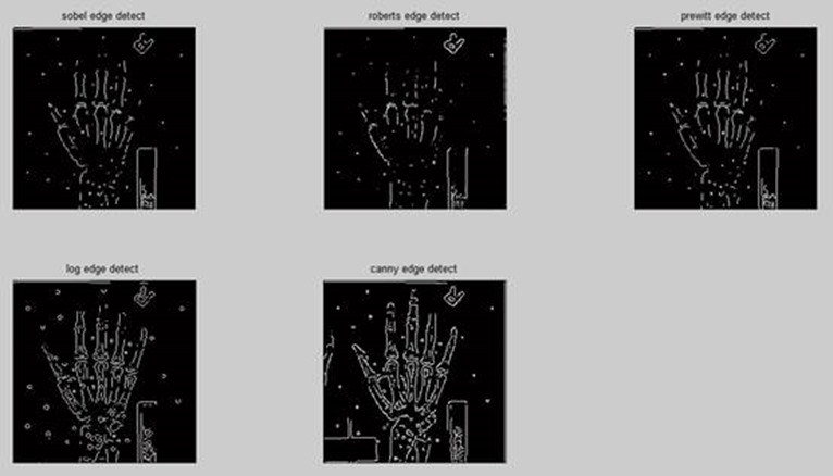
- The Sobel operator detection method has a better processing effect on images with gray gradients and more noise. The Sobel operator is not very accurate in edge positioning, and the edge of the image is more than one pixel;
- The Roberts operator detection method has a better processing effect on images with steep low noise, but the result of using the Roberts operator to extract edges is that the edges are relatively thick, so the edge positioning is not very accurate;
- The Prewitt operator detection method has better processing effects on images with grayscale gradients and more noise. But the edges are wider and have many discontinuities;
- The Laplacian operator method is relatively sensitive to noise, so this operator is rarely used to detect edges. Instead, it is used to determine whether edge pixels are regarded as bright or dark areas of the image;
- The Canny method is not susceptible to noise interference and can detect real weak edges. The advantage is that two different thresholds are used to detect strong edges and weak edges respectively, and only when the weak edges and strong edges are connected, the weak edges are included in the output image.
2. Edge composite enhancement
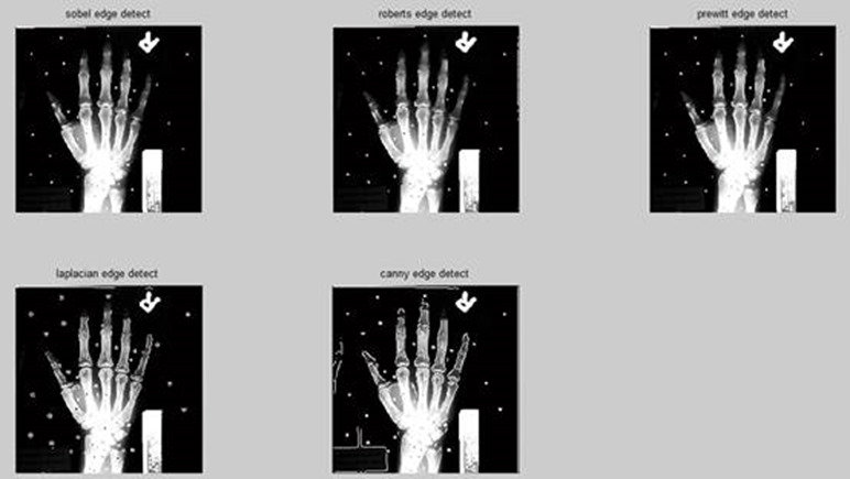
- The enhancement effects of the Sobel, Robert, and Prewitt operators are not very obvious, especially the Robert operator, because the edge points it extracts are too sparse and discrete;
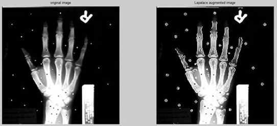
- The enhancement effects of the Laplacian operator and the canny operator are both ideal. After superimposing the edges, the outline and edges of the entire hand are very clear. Intuitively, the effect achieved by the canny operator is better than that of the Laplacian operator. The most obvious thing is It’s the edge of your fingertips.
- Image edge detection based on ant colony algorithm
3. Program implementation
The following program is the complete Matlab code to achieve the above effect:
clear;clc;
I=imread('x1.tif');
% I=rgb2gray(I);
% gray transform

J=imadjust(I,[0.1 0.9],[0 1],1);

% Edge detection
% Sobel
BW1=edge(I,'sobel');
sobelBW1=im2uint8(BW1) + J;
figure;
%imshow(BW1);
subplot(1,2,1);
imshow(J);
title('original image');
subplot(1,2,2);
imshow(sobelBW1);
title('Sobel augmented image');
%Roberts
BW2=edge(I,'roberts');
robertBW2=im2uint8(BW2) + J;
figure;
%imshow(BW2);
subplot(1,2,1);
imshow(J);
title('original image');
subplot(1,2,2);
imshow(robertBW2);
title('robert augmented image');
% prewitt
BW3=edge(I,'prewitt');
prewittBW3=im2uint8(BW3) + J;
figure;
%imshow(BW3);
subplot(1,2,1);
imshow(J);
title('original image');
subplot(1,2,2);
imshow(prewittBW3);
title('Prewitt augmented image');
%log
BW4=edge(I,'log');
logBW4=im2uint8(BW4) + J;
figure;
%imshow(BW4);
subplot(1,2,1);
imshow(J);
title('original image');
subplot(1,2,2);
imshow(logBW4);
title('Laplacian augmented image');
% canny
BW5=edge(I,'canny');
cannyBW5=im2uint8(BW5) + J;
figure;
%imshow(BW5);
subplot(1,2,1);
imshow(J);
title('original image');
subplot(1,2,2);
imshow(cannyBW5);
title('Canny augmented image');
% gaussian & canny
% h=fspecial('gaussian',5);
% fI=imfilter(I,h,'replicate');
% BW6=edge(fI,'canny');
% figure;
% imshow(BW6);

figure;
subplot(2,3,1), imshow(BW1);
title('sobel edge detect');
subplot(2,3,2), imshow(BW2);
title('roberts edge detect');
subplot(2,3,3), imshow(BW3);
title('prewitt edge detect');
subplot(2,3,4), imshow(BW4);
title('log edge detect');
subplot(2,3,5), imshow(BW5);
title('canny edge detect');
% subplot(2,3,6), imshow(BW6);
% title('gasussian & amp;canny edge detect');

figure;
subplot(2,3,1), imshow(sobelBW1);
title('sobel edge detect');
subplot(2,3,2), imshow(robertBW2);
title('roberts edge detect');
subplot(2,3,3), imshow(prewittBW3);
title('prewitt edge detect');
subplot(2,3,4), imshow(logBW4);
title('laplacian edge detect');
subplot(2,3,5), imshow(cannyBW5);
title('canny edge detect');
The following Matlab program is a streamlined edge extraction implementation:
clear;clc;

I=imread('lena.bmp');
I=rgb2gray(I);
imshow(I,[]);
title('Original Image');

sobelBW=edge(I,'sobel');
figure;
imshow(sobelBW);
title('Sobel Edge');

robertsBW=edge(I,'roberts');
figure;
imshow(robertsBW);
title('Roberts Edge');

prewittBW=edge(I,'prewitt');
figure;
imshow(prewittBW);
title('Prewitt Edge');

logBW=edge(I,'log');
figure;
imshow(logBW);
title('Laplasian of Gaussian Edge');

cannyBW=edge(I,'canny');
figure;
imshow(cannyBW);
title('Canny Edge');
The knowledge points of the article match the official knowledge files, and you can further learn related knowledge. OpenCV skill tree Home page Overview 24004 people are learning the system