Table of Contents
1. pmdarima implements univariate time series forecasting
2. Time series cross-validation
2.1 Rolling Cross Validation (RollingForecastCV)
2.2 Sliding window cross-validation (SildingWindowForecastCV)
1. pmdarima implements univariate time series prediction
Pmdarima is a Python timing analysis library developed and encapsulated based on statsmodel and autoarima. It is also one of the timing prediction libraries with the highest degree of encapsulation and the simplest code on the market. Pmdarima was developed by the sklearn team. It follows the coding habits of the sklearn library and retains all interfaces to sklearn. It is a very convenient tool for machine learning learners. This library includes all the functions of autoarima based on the R language, and can handle issues such as stationarity, seasonality, and periodicity. It can perform operations such as differences and cross-validation, as well as rich official documentation. The following is the process of using Pmdarima to implement a simple prediction:
import pmdarima as pm
from pmdarima import model_selection
import numpy as np
import pandas as pd
import matplotlib.pyplot as plt
from sklearn.metrics import mean_squared_error
import warnings
warnings.filterwarnings("ignore")

data = pm.datasets.load_wineind()
len(data) #176

fig=plt.figure(figsize=(16,5))
plt.plot(range(data.shape[0]),data)
plt.grid()

#Use pm to split data and follow timing rules without disrupting the time sequence.
train, test = model_selection.train_test_split(data, train_size=152)
#Automated modeling, only supports SARIMAX hybrid models, does not support VARMAX series models
arima = pm.auto_arima(train, trace=True, #Training data, do you want to print the training process?
                      error_action='ignore', suppress_warnings=True, #Ignore warnings and errors
                      maxiter=5, #Maximum number of iterations allowed
                      seasonal=True, m=12 #Should we use seasonal factors? If used, what is the number of steps for multi-step prediction?
                     )
Performing stepwise search to minimize aic
 ARIMA(2,1,2)(1,0,1)[12] intercept : AIC=2955.247, Time=0.46 sec
 ARIMA(0,1,0)(0,0,0)[12] intercept : AIC=3090.160, Time=0.02 sec
 ARIMA(1,1,0)(1,0,0)[12] intercept : AIC=2993.480, Time=0.08 sec
 ARIMA(0,1,1)(0,0,1)[12] intercept : AIC=2985.395, Time=0.09 sec
 ARIMA(0,1,0)(0,0,0)[12] : AIC=3088.177, Time=0.02 sec
 ARIMA(2,1,2)(0,0,1)[12] intercept : AIC=2978.426, Time=0.16 sec
 ARIMA(2,1,2)(1,0,0)[12] intercept : AIC=2954.744, Time=0.18 sec
 ARIMA(2,1,2)(0,0,0)[12] intercept : AIC=3025.510, Time=0.10 sec
 ARIMA(2,1,2)(2,0,0)[12] intercept : AIC=2954.236, Time=0.49 sec
 ARIMA(2,1,2)(2,0,1)[12] intercept : AIC=2958.264, Time=0.49 sec
 ARIMA(1,1,2)(2,0,0)[12] intercept : AIC=2964.588, Time=0.38 sec
 ARIMA(2,1,1)(2,0,0)[12] intercept : AIC=2950.034, Time=0.53 sec
 ARIMA(2,1,1)(1,0,0)[12] intercept : AIC=2950.338, Time=0.24 sec
 ARIMA(2,1,1)(2,0,1)[12] intercept : AIC=2953.291, Time=0.45 sec
 ARIMA(2,1,1)(1,0,1)[12] intercept : AIC=2951.569, Time=0.21 sec
 ARIMA(1,1,1)(2,0,0)[12] intercept : AIC=2958.953, Time=0.32 sec
 ARIMA(2,1,0)(2,0,0)[12] intercept : AIC=2966.286, Time=0.35 sec
 ARIMA(3,1,1)(2,0,0)[12] intercept : AIC=2951.433, Time=0.50 sec
 ARIMA(1,1,0)(2,0,0)[12] intercept : AIC=2993.310, Time=0.39 sec
 ARIMA(3,1,0)(2,0,0)[12] intercept : AIC=2952.990, Time=0.47 sec
 ARIMA(3,1,2)(2,0,0)[12] intercept : AIC=2953.842, Time=0.58 sec
 ARIMA(2,1,1)(2,0,0)[12] : AIC=2946.471, Time=0.45 sec
 ARIMA(2,1,1)(1,0,0)[12] : AIC=2947.171, Time=0.17 sec
 ARIMA(2,1,1)(2,0,1)[12] : AIC=2948.216, Time=0.42 sec
 ARIMA(2,1,1)(1,0,1)[12] : AIC=2946.151, Time=0.29 sec
 ARIMA(2,1,1)(0,0,1)[12] : AIC=2971.736, Time=0.14 sec
 ARIMA(2,1,1)(1,0,2)[12] : AIC=2948.085, Time=0.50 sec
 ARIMA(2,1,1)(0,0,0)[12] : AIC=3019.258, Time=0.06 sec
 ARIMA(2,1,1)(0,0,2)[12] : AIC=2959.185, Time=0.36 sec
 ARIMA(2,1,1)(2,0,2)[12] : AIC=2950.098, Time=0.52 sec
 ARIMA(1,1,1)(1,0,1)[12] : AIC=2953.184, Time=0.14 sec
 ARIMA(2,1,0)(1,0,1)[12] : AIC=2964.069, Time=0.14 sec
 ARIMA(3,1,1)(1,0,1)[12] : AIC=2949.076, Time=0.16 sec
 ARIMA(2,1,2)(1,0,1)[12] : AIC=2951.826, Time=0.16 sec
 ARIMA(1,1,0)(1,0,1)[12] : AIC=2991.086, Time=0.09 sec
 ARIMA(1,1,2)(1,0,1)[12] : AIC=2960.917, Time=0.14 sec
 ARIMA(3,1,0)(1,0,1)[12] : AIC=2950.719, Time=0.13 sec
 ARIMA(3,1,2)(1,0,1)[12] : AIC=2952.019, Time=0.17 sec

Best model: ARIMA(2,1,1)(1,0,1)[12]
Total fit time: 11.698 seconds
#Prediction
preds = arima.predict(n_periods=test.shape[0])
preds #Predict based on the date of the test set
array([25809.09822027, 27111.50500611, 30145.84346715, 35069.09860267,
       19044.09098919, 22734.07766136, 24370.14476344, 24468.4989244,
       24661.71940304, 24465.6250753, 29285.02123954, 25607.32326197,
       26131.79439226, 26937.20321329, 29632.82588046, 33904.51565498,
       20207.31393733, 23342.10936251, 24741.41755828, 24828.6385991,
       24993.22466868, 24825.14042152, 28939.23990247, 25799.92370898])
fig=plt.figure(figsize=(16,5))
plt.plot(range(test.shape[0]),test)
plt.plot(range(test.shape[0]),preds)
plt.grid()

Model evaluation indicators can share the evaluation indicators of sklearn, or call specific time series indicators AIC:
np.sqrt(mean_squared_error(test, preds))
2550.8826581401277
arima.aic()
2946.1506587436375
arima.summary()

Enumeration-based search for appropriate parameters is far more efficient than statsmodel. Unfortunately, from the above code, it is not difficult to see that the code idea of pmdarima is more recent machine learning than statistics, so pmd.auto arima ran out The results often fail to meet various statistical testing requirements, so the generalization ability cannot be guaranteed. At the same time, it is easy to find that due to the division of the data set, the best model selected by autoarima may not be reproduced. For example, we use the best model selected by autoarima to establish a single model:
model=pm.ARIMA(order=(2,1,1),seasonal_order=(1,0,1,12),max_iter=500)
model.fit(train)

fig=plt.figure(figsize=(16,5))
plt.plot(range(test.shape[0]),test)
plt.plot(range(test.shape[0]),model.predict(n_periods=test.shape[0]))
plt.grid()

np.sqrt(mean_squared_error(test, model.predict(n_periods=test.shape[0])))
3081.3401428137163
model.aic()
2936.648256262213
Since pmdarima is built based on statsmodel, it can also use all the functions of autoarima based on R language. pmdarima can naturally also support corresponding various statistical tests and correlation coefficient calculations. For more details, please refer to the official documentation of pmdarima. Generally, after using pmdarima for modeling, you need to use a series of tests in statistics to select a model and find a model that can pass all tests.
2. Time series cross-validation
In the selection process of time series models, we can use cross-validation to help us choose a better model. Time series cross-validation is very special, because time series data must abide by the basic principles of “predicting the future from the past” and “the time sequence cannot be disrupted during training”, so k-fold cross-validation in traditional machine learning cannot be used.
In the world of time series, there are two common cross-validation methods: rolling cross-validation (RollingForecastCV) and sliding window cross-validation (SlidingWindowForecastCV). When “time-series cross-validation” is mentioned, rolling cross-validation is generally referred to. Let’s take a closer look at the two cross-validation operations:
2.1 Rolling Cross Validation (RollingForecastCV)

Rolling cross-validation is a verification method that continuously increases the training set during the verification process and moves the verification set closer and closer to the future. This method can not only ensure that we are using the past to predict the future, but also ensure that we need to predict The distance between the real labels in the future and the past is close enough, because the closer the future data is, the greater the impact on the future. This cross-validation method is very similar to “multi-step prediction”, but this method does not have the “error accumulation” problem in multi-step prediction, because we have been using objectively existing real labels during the training process.
In pmdarima, we use the classes RollingForecastCV and cross_validate to implement cross-validation. It is obvious that pmdarima’s ideas are borrowed from sklearn (in fact, pmdarima draws on and relies on statsmodel for all statistics-related content, and relies on statsmodel for all machine learning-related content. The above is based on sklearn for operation). Cross validation in sklearn:
cv = KFold(n_splits=5,shuffle=True,random_state=1412)
results = cross_validate(reg,Xtrain,Ytrain,cv=cv)
Among them, cv is the specific mode of cross-validation, and cross_validate is responsible for executing the cross-validation itself. When running cross-validation in pmdarima, the status of class RollingForecastCV is equivalent to the KFold class in ordinary machine learning cross-validation. RollingForecastCv can only specify the cross-validation mode and is not responsible for performing cross-validation itself. In particular, ordinary K-fold cross-validation is controlled by the number of folds, but sequential cross-validation is actually based on a single sample. Generally speaking, the validation set of time series cross-validation can be multiple time points or a single time point. When the validation set is 1 time point, rolling cross-validation looks like this:

In pmdarima, use RollingForecastCV to complete cross-validation:
class pmdarima.model selection.RollingForecastCV(h=1, step=1, initial=None)
h: The number of samples in the validation set, you can enter an integer of [1,n_samples].
step: The number of samples added to the training set each time, must be a positive integer greater than or equal to 1.
initial: The training set sample size in the first cross-validation. If not filled in, it will be processed as 1/3.
Take h=1, step=1, initial=10
data = pm.datasets.load_wineind()
cv=model_selection.RollingForecastCV(h=1,step=1,initial=10)
cv_generator=cv.split(data)
next(cv_generator)# According to the initial initial training set, there are 10 samples, and the verification set follows the setting of parameter h and only contains one sample
(array([0, 1, 2, 3, 4, 5, 6, 7, 8, 9]), array([10]))
next(cv_generator)#According to the setting of step, the training set increases by 1 sample each time, and the verification set continues to contain one sample
(array([ 0, 1, 2, 3, 4, 5, 6, 7, 8, 9, 10]), array([11]))
next(cv_generator)
(array([ 0, 1, 2, 3, 4, 5, 6, 7, 8, 9, 10, 11]), array([12]))
Take h=10, step=5, initial=10
cv=model_selection.RollingForecastCV(h=10,step=5,initial=10)
cv_generator=cv.split(data)
next(cv_generator)
(array([0, 1, 2, 3, 4, 5, 6, 7, 8, 9]),
 array([10, 11, 12, 13, 14, 15, 16, 17, 18, 19]))
next(cv_generator)
(array([ 0, 1, 2, 3, 4, 5, 6, 7, 8, 9, 10, 11, 12, 13, 14]),
 array([15, 16, 17, 18, 19, 20, 21, 22, 23, 24]))
next(cv_generator)
(array([ 0, 1, 2, 3, 4, 5, 6, 7, 8, 9, 10, 11, 12, 13, 14, 15, 16,
        17, 18, 19]),
 array([20, 21, 22, 23, 24, 25, 26, 27, 28, 29]))
It is not difficult to find that when rolling cross-validation is implemented in pmdarima, the verification set can actually be repeated. Therefore, rolling cross-validation can perform multiple rounds of cross-validation with overlapping verification sets on limited data, as long as the “past predicts the future” condition is met. As a basic rule, temporal cross-validation can actually be performed relatively freely (that is, the validation set and the validation set are not mutually exclusive). Therefore, the actual running time of sequential cross-validation is often very long, and the burden of cross-validation will be greater when the amount of data is huge.
# Use the above data and model
model=pm.ARIMA(order=(2,1,1),seasonal_order=(1,0,1,12),max_iter=500)
cv=model_selection.RollingForecastCV(h=24,step=12,initial=36)
predictions=model_selection.cross_validate(model,data,cv=cv
                                            ,scoring="mean_squared_error"
                                            ,verbose=2
                                            ,error_score="raise")
[CV] fold=0 ........................................ .....................
[CV] fold=1 ........................................ ............
[CV] fold=2 ........................................ ............
[CV] fold=3 ........................................ ............
[CV] fold=4 ........................................ ............
[CV] fold=5 ........................................ ............
[CV] fold=6 ........................................ ............
[CV] fold=7 ........................................ ............
[CV] fold=8 ........................................ ............
[CV] fold=9 ........................................ ............
predictions
{'test_score': array([1.35362847e + 08, 1.08110482e + 08, 2.18376249e + 07, 1.97805181e + 07,
        6.16138893e + 07, 1.42418110e + 07, 1.32432958e + 07, 1.31182597e + 07,
        3.57071218e + 07, 5.79654872e + 06]),
 'fit_time': array([0.2784729 , 0.12543654, 0.62335014, 0.64258695, 0.75659704,
        0.73791075, 0.82430649, 0.92007995, 0.98767185, 1.03166628]),
 'score_time': array([0.01047397, 0. , 0.00223732, 0. , 0. ,
        0. , 0.01564431, 0. , 0.01562428, 0.01562572])}
np.sqrt(predictions["test_score"])
array([11634.55400113, 10397.61906654, 4673.07446159, 4447.52944078,
        7849.45153132, 3773.83240719, 3639.13393689, 3621.91381986,
        5975.54363899, 2407.60227639])
It can be seen that most of the RMSE obtained in the cross-validation test set is greater than the RMSE (2550) obtained in the previous automated modeling, and when the training data is less, the RMSE on the test set will be larger, which may indicate that in the first few days During fold cross-validation, the amount of data in the training set is too small, so you can consider increasing the settings in the initial to avoid this problem.
2.2 Sliding Window Cross Validation (SildingWindowForecastCV)
Sliding window cross-validation is a cross-validation completed with the help of sliding window technique. Sliding window is a common technique in time series. The specific operation is as follows:
Sliding window–>–>
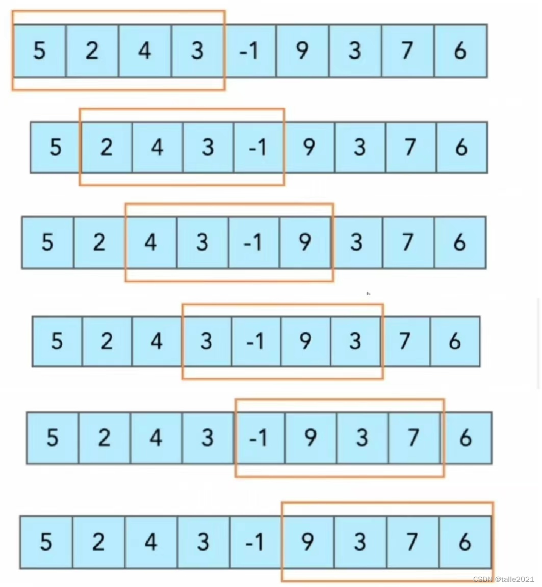
In time series prediction, the samples within the window are often used as training samples, and the first sample on the right side (or below) of the window is used as the predicted sample. The sliding window technique is widely used in various fields of time series and is one of the foundations of time series. Obviously, sliding window cross-validation is cross-validation using the samples within the window as the training set and the samples on the right (or below) of the window as the validation set.

Like rolling cross-validation, the validation set in sliding window cross-validation can also be a single sample or a series of data sets. Compared with rolling cross-validation, the advantage of sliding window cross-validation is that the training set does not become larger and larger, and each training uses the most effective information in theory for the current validation set. But at the same time, this advantage also brings problems. Since the training set is often small, sliding window cross-validation requires an unusually large number of modeling times, which may cause the cross-validation model to become very slow.
In pmdarima, use SlidingWindowForecastCV to complete sliding window cross-validation
class pmdarima.model_selection.SlidingWindowForecastCV(h=1,step=1,window size=None)
h: The number of samples in the validation set, you can enter an integer of [1,n_samples]
step: The number of samples for each sliding window to the future, must be a positive integer greater than or equal to 1
window_size: The size of the sliding window. If you fill in None, it will be determined by the number obtained by dividing the sample size by 5.
Take h=1, step=1, window_size=10
cv=model_selection.SlidingWindowForecastCV(h=1,step=1,window_size=10)
cv_generator=cv.split(data)
next(cv_generator)#Data splitting during the first cross-validation
(array([0, 1, 2, 3, 4, 5, 6, 7, 8, 9]), array([10]))
next(cv_generator)#Data segmentation during the second cross-validation
(array([ 1, 2, 3, 4, 5, 6, 7, 8, 9, 10]), array([11]))
Take h=10, step=5, window_size=10
cv=model_selection.SlidingWindowForecastCV(h=10,step=5,window_size=10)
cv_generator=cv.split(data)
next(cv_generator)
(array([0, 1, 2, 3, 4, 5, 6, 7, 8, 9]),
 array([10, 11, 12, 13, 14, 15, 16, 17, 18, 19]))
next(cv_generator)
(array([ 5, 6, 7, 8, 9, 10, 11, 12, 13, 14]),
 array([15, 16, 17, 18, 19, 20, 21, 22, 23, 24]))
# Use the above data and model
model=pm.ARIMA(order=(2,1,1),seasonal_order=(1,0,1,12),max_iter=500)
cv=model_selection.SlidingWindowForecastCV(h=24,step=12,window_size=36)
predictions=model_selection.cross_validate(model,data,cv=cv
                                            ,scoring="mean_squared_error"
                                            ,verbose=2
                                            ,error_score="raise")
[CV] fold=0 ........................................ .....................
[CV] fold=1 ........................................ ............
[CV] fold=2 ........................................ ............
[CV] fold=3 ........................................ ............
[CV] fold=4 ........................................ ............
[CV] fold=5 ........................................ ............
[CV] fold=6 ........................................ ............
[CV] fold=7 ........................................ ............
[CV] fold=8 ........................................ ............
[CV] fold=9 ........................................ ............
predictions
{'test_score': array([1.35362847e + 08, 1.20867167e + 08, 1.48347243e + 08, 2.49879706e + 08,
        2.32217899e + 08, 4.01511152e + 08, 1.92061264e + 08, 2.51755311e + 08,
        1.50798724e + 08, 1.92747682e + 08]),
 'fit_time': array([0.28506732, 0.16709971, 0.17653751, 0.12498903, 0.1408143,
        0.16088152, 0.22708297, 0.33786058, 0.1593399, 0.27807832]),
 'score_time': array([0.00801778, 0. , 0.01562667, 0. , 0.01132369,
        0. , 0.01562595, 0. , 0.01562929, 0. ])}
np.sqrt(predictions["test_score"])
array([11634.55400113, 10993.96047191, 12179.78831408, 15807.58382521,
       15238.69740534, 20037.7431982, 13858.61697326, 15866.79900091,
       12280.01317219, 13883.35991075])
Judging from the results, after using fewer training sets for training, the RMSE of the model output increased significantly and did not become more stable. This shows that a larger training set under the current model is more conducive to model training (not every This is true for every time series). Try adjusting the window_size of the sliding window, and you will find that the RMSE drops to a level similar to that of rolling cross-validation:
model=pm.ARIMA(order=(2,1,1),seasonal_order=(1,0,1,12),max_iter=500)
cv=model_selection.SlidingWindowForecastCV(h=24,step=1,window_size=132)
predictions=model_selection.cross_validate(model,data,cv=cv
                                            ,scoring="mean_squared_error"
                                            ,verbose=2
                                            ,error_score="raise")
[CV] fold=0 ........................................ .....................
[CV] fold=1 ........................................ ............
[CV] fold=2 ........................................ ............
[CV] fold=3 ........................................ ............
[CV] fold=4 ........................................ ............
[CV] fold=5 ........................................ ............
[CV] fold=6 ........................................ ............
[CV] fold=7 ........................................ ............
[CV] fold=8 ........................................ ............
[CV] fold=9 ........................................ ............
[CV] fold=10 ........................................ .............
[CV] fold=11 ........................................ .............
[CV] fold=12 ........................................ .............
[CV] fold=13 ........................................ .............
[CV] fold=14 ........................................ .............
[CV] fold=15 ........................................ .............
[CV] fold=16 ........................................ .............
[CV] fold=17 ........................................ .............
[CV] fold=18 ........................................ .............
[CV] fold=19 ........................................ .............
[CV] fold=20 ........................................ .............
predictions
{'test_score': array([35707121.78143389, 66176325.69903485, 40630659.97659013,
        78576782.28645307, 23666490.55159284, 20310751.60353827,
         2841898.1720445, 4484619.0619739, 18925627.1367884,
         3231920.46993413, 55955063.23334328, 5769421.1274077,
        12204785.2577201, 81763866.37114508, 86166090.62031393,
         4308494.01384212, 4472068.45984436, 80544390.23157245,
        95444224.35956413, 4356301.4101477, 41312817.67528097]),
 'fit_time': array([0.98685646, 1.00776458, 0.98309445, 0.98523855, 0.99820113,
        0.88483882, 1.14556432, 0.94388413, 0.95140123, 1.01311779,
        1.01590633, 1.06021142, 1.05152464, 1.06878543, 1.08534598,
        1.07379961, 0.96942186, 0.92225981, 0.95834565, 1.33569884,
        0.91161823]),
 'score_time': array([0.01562262, 0.01562762, 0. , 0.00460625, 0. ,
        0.00678897, 0.00810504, 0.01536226, 0.01825047, 0.00629425,
        0.00742435, 0.01564217, 0. , 0. , 0. ,
        0. , 0.00800204, 0.01618385, 0. , 0.01562595,
        0. ])}
np.sqrt(predictions["test_score"])
array([5975.54363899, 8134.88326278, 6374.21838162, 8864.35458939,
       4864.82173893, 4506.74512298, 1685.79303951, 2117.69191857,
       4350.35942616, 1797.75428519, 7480.31170696, 2401.96193296,
       3493.53477981, 9042.33743958, 9282.56918209, 2075.69121351,
       2114.72656858, 8974.65265242, 9769.55599603, 2087.17546223,
       6427.50477832])
At this time, the mean value of RMSE has dropped significantly, but the model is still unstable (large fluctuations), which shows that the differences in each time period of the current time series are large, and the fitting results of the current model are average. Although the performance of the model can be improved by increasing the amount of data in the training set, the extremely unstable results demonstrate that the generalization ability of the current model is lacking. Just like when using AIC, we can only choose a timing model with better performance (only the best), but cannot choose a perfect timing model. When we give up the best parameters selected by auto_arima and choose a model with other parameters, the results may be more unstable.
Did you notice a detail? Temporal cross-validation does not return scores on the training set, and pmdarima’s prediction function predict does not accept predictions into the past. Generally speaking, our criterion for judging overfitting is that the results on the training set are much better than the test set. However, time series cross-validation does not return the training set score, so time series data cannot be judged by comparing the results of the training set and the test set. Overfitting. But in the world of time series, the concept of “overfitting” still exists. We can use the results of cross-validation to determine which time series model under different parameters has a lighter degree of overfitting.
Generally speaking, the model with the best score on the validation set tends to have the smallest risk of overfitting, because when a model learning can be strong enough and is neither overfitting nor underfitting, the training set and validation set scores of the model will It should be highly close, so the better the validation set score, the more likely it is that the validation set score will be closer to the score on the training set. Therefore, in the case of multiple model comparisons, we can select the best model just by observing the scores on the test set. This best model is the model with the best performance and the model with the smallest risk of overfitting (not absolute).