Hands-on implementation of deep neural network 1 two-layer neural network
In this series, we will try to use python to write a neural network. Of course, the actual neural network model available is not very complicated, involving many implementation details and optimizations. Therefore, we will start with a two-layer neural network, and then Continuous improvement and improvement.
We use this network for handwritten digit recognition in the MNIST dataset. Because this is the first network, it is relatively simple in advance. Batch processing is not implemented, but one image is input each time (when a handwritten image in the MNIST dataset is entered) 28*28 matrix, for the convenience of operation, we generally flatten it into a one-dimensional matrix with 784 elements). At the same time, because the method of numerical differentiation is used in calculating the gradient, it is very slow, so both the training data and the test data can only be selected from a small part of the MNIST data set. But don’t get discouraged, a fast and efficient neural network will be implemented in the next article.
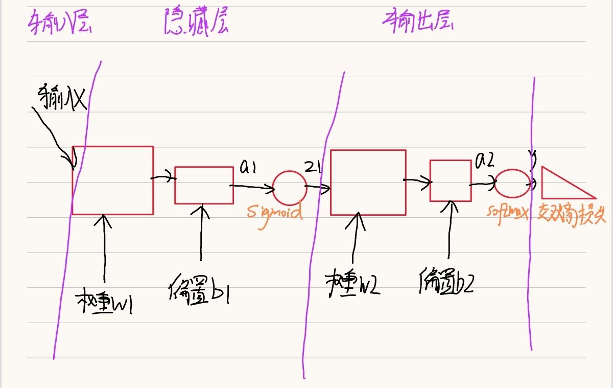
1. The basic structure of the network
2. Class of two-layer neural network
2.1 Defining classes and class initialization functions
class Myself_Two_Layer_Net:
    # A neural network should accept some hyperparameter settings during initialization, such as: the number of neurons in each layer, the size of the Gaussian distribution when initializing parameters
    def __init__(self, input_size, hidden_size, output_size, weight_init_std):
        # This is the parameter of the neural network, which is stored in a dictionary
        # parameter initialization
        self.params={}
        # w1 b1 are the weights and biases of the first layer (hidden layer)
        # The shape of w1 is a matrix of input_size*hidden_size The shape of b1 is a one-dimensional matrix with hidden_size elements
        # When the parameters are generally initialized, Gaussian distribution (normal distribution) random numbers are selected np.random.randn(a,b) to generate a random number matrix with a row and b column that conforms to the Gaussian distribution
        self.params['w1']=weight_init_std*np.random.randn(input_size,hidden_size)
        self.params['b1']=np.zeros(hidden_size)
        # w2 b2 is the weight and bias of the second layer (hidden layer)
        self.params['w2'] = weight_init_std * np.random.randn(hidden_size,output_size)
        self.params['b2'] = np.zeros(output_size)
A neural network should accept some hyperparameter settings during initialization, such as: number of neurons in each layer, parameter initialization rules, etc. Since the work of “tuning parameters according to gradients” is not placed in this class, there is no need to accept learning rate.
Parameter initialization generally uses Gaussian distribution random initialization. The specific value of the number of neurons in each layer will be explained later when this network is used.
2.2 Workflow of Two-Layer Neural Network
1 Receive input –>2 After two layers of operations –>3 Find the loss function value –>4 Find the gradient of the loss function value with respect to each parameter –>5 (update the parameters according to the gradient)
Step 1 has been implemented in the “class initialization method”, and step 5 is implemented by the user of the class. Therefore, it is mainly to achieve 2 3 4 three steps.
2.2.1 goes through two layers of operations
# After two layers of operations
def predict(self,x):
# get parameters
w1,b1=self.params['w1'],self.params['b1']
w2,b2=self.params['w2'],self.params['b2']
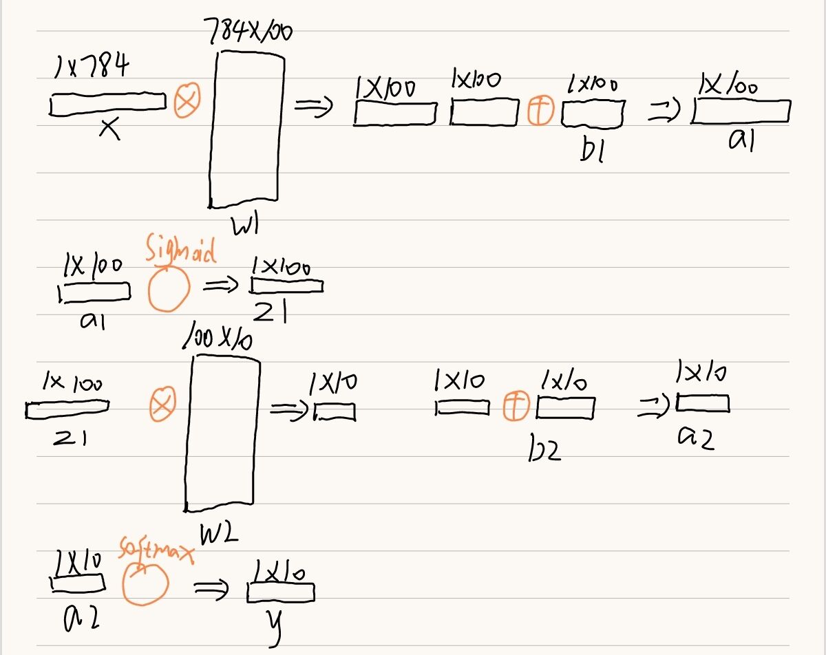
a1=np.dot(x,w1) + b1
# Here we need to implement the sigmoid activation function ourselves
z1=sigmoid(a1)
a2=np.dot(z1,w2) + b2
# Here we need to implement the softmax activation function ourselves
y=softmax(a2)
return y
It can be seen that the calculation process of the neural network is still very simple. We use np.dot for matrix multiplication.
We need to implement the two activation functions of sigmoid and softmax by ourselves (if you are not familiar with these two activation functions, you can read my previous article for a detailed explanation)
def sigmoid(x):
    # Use np.exp instead of math.exp because it is a matrix operation
    return 1/(1 + np.exp(-x))
def softmax(x):
    max=np.max(x)
    x=x-max
    return np.exp(x)/np.sum(np.exp(x))
(The softmax function here is only used with a neural network that does not implement batch processing, and it will be improved in subsequent articles)
“ max=np.max(x)
x=x-max ”
These two lines of code are to prevent calculation overflow. Here are two questions to answer:
1. Why does calculation overflow occur?
Because the implementation of the softmax function requires the operation of the exponential function, but the value of the exponential function can easily become very large. For example, the value of exp(10) will exceed 20000, exp(100) will become an oversized value with more than 40 zeros behind it, and the result of exp(1000) will return an inf representing infinity. If you divide between these very large values, the result will be “indeterminate”.
2. Why is it possible to use such a simple and crude function as subtracting the maximum value?
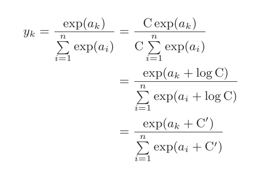
It can be seen from this formula that adding (or subtracting) a constant will not change the result of the operation when performing the exponential function of softmax..
2.2.2 Find the value of the loss function
# Find the value of the loss function
def loss(self,x,t):
    y=self.predict(x)
    # Here we need to implement the cross entropy loss function ourselves
    return cross_entropy_error(y,t)
# Cross entropy function without batch learning Supervised data is in one-hot format
# For the case where the supervision data is in one-hot format, only the natural logarithm of the output corresponding to the correct solution label is actually calculated
def cross_entropy_error(y,t):
    # When calculating np.log inside the function, a tiny value delta 1e-7 is added.
    # This is because, when np.log(0) occurs, np.log(0) will become negative infinity - inf, which will make subsequent calculations impossible. As a protective countermeasure, adding a tiny value prevents negative infinity from happening
    delta=1e-7
    return -np.sum(t*np.log(y + delta))
Two questions are explained here:
One is supervised data. It is easy to confuse the concept of test data, and the code behind will give you a more intuitive understanding

One is in one-hot format (one-hot encoding), which means that set the correct solution tag to 1, the others are set to 0
Assume the supervised data t is [0,0,1,0,0,0,0,0,0,0] The output y of the neural network is [0.1,0.05,0.6,0.1…] The index of the correct solution label is “2”, and the corresponding output of the neural network is 0.6
Then the cross entropy is: it is?log 0.6 = 0.51
Let’s write an example to verify:
t=np.array([0,0,1,0,0,0,0,0,0,0])
# The key here is that index 2 is 0.6, other location data is not important
y=np.array([0.1,0.05,0.6,0.05,0.05,0.05,0.01,0.01,0.02,0.06])
print(np.log(y))
print(t*np.log(y))
z=-np.sum(t*np.log(y))
print(z)
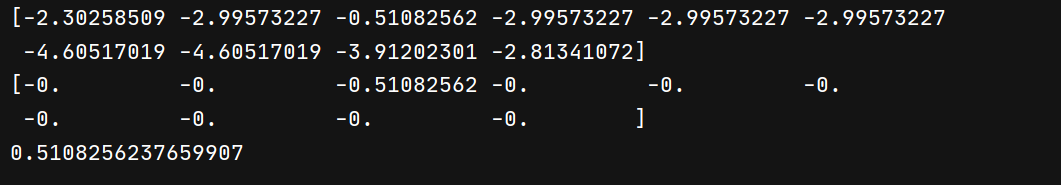
Therefore, it can be said that the value of the cross-entropy error is determined by the output corresponding to the correct solution label.
2.2.3 Find the gradient of a loss function value with respect to each parameter
# Find the gradient of the loss function value with respect to each parameter
def gradient_numerical(self,x,t):
    # Pass the first two steps of operations to form a lambda expression (which can be understood as a mathematical function) to the method that calculates the gradient
    loss_W=lambda w:self.loss(x,t)

    grads={}
    # Here we need to implement numerical_gradient by ourselves (calculate gradient with numerical differential distribution)
    grads['w1'] = numerical_gradient_2d(loss_W, self.params['w1'])
    grads['b1'] = numerical_gradient_2d(loss_W, self.params['b1'])
    grads['w2'] = numerical_gradient_2d(loss_W, self.params['w2'])
    grads['b2'] = numerical_gradient_2d(loss_W, self.params['b2'])

    return grads
# The independent variable x can only be a one-dimensional matrix, that is, the bias b
def numerical_gradient_1d(f, x):
    h = 1e-4
    grad = np.zeros_like(x)

    # x is [x1,x2,.....] f is f(x1,x2,.....)
    for i in range(x.size):
        temp=x[i]
        x[i]=x[i] + h
        fxh1=f(x) # Calculate f(x + h) Because it is a multivariate function, only xi plus h is not added to other x

        x[i]=temp
        x[i]=x[i]-h
        fxh2=f(x)

        grad[i]=(fxh1 + fxh2)/2

        x[i]=temp

    return grad

# Both the two-dimensional matrix w and the one-dimensional matrix b can be
def numerical_gradient_2d(f, x):
    if x.ndim == 1:
        return numerical_gradient_1d(f, x)
    else:
        grad = np.zeros_like(x)

        for i, x_i in enumerate(x):
            grad[i] = numerical_gradient_1d(f, x_i)

        return grad
What needs to be explained here are:
One, because the bias b is a one-dimensional number, and the weight w is a matrix, the gradient of the weight w needs to be calculated line by line in the loop.
Second, lambda expression, loss_W=lambda w:self.loss(x,t) This line of code encapsulates the first two steps as a lambda function, which can be passed to other methods as parameters.
It can be seen that the parameter ‘w’ in this lambda function formula is not very useful, and it is not passed into the parameter at all.
That is to say, the line of code “fxh1 = f(x)” can be written as “fxh1 = f(1) fxh1 = f(2)” or pass any number to the parameter of f. Because what really works is "x = x + h" and "x = temp - h"they change the value in params! ! , after calling f(), the two lines of code “y=self.predict(x) return cross_entropy_error(y,t)” will be executed, and the params used in self.predict have been modified, so you can Get the function value at x + h.
Write an example below to verify:
def add(x,y):
    return x + y

def use(f, a):
    z1=f(a)
    print(z1)

afunction = lambda w: add(1, 2)
use(afunction,5)
use(afunction,6)
use(afunction,100)
3. The use of two-layer neural network
At this point, our simple two-layer neural network class has been written, and the next step is to use it. But once again, this neural network design is simple and does not implement batch processing, and does not use error backpropagation to calculate gradients. The efficiency is very, very low. Here is just an introduction to the use process. It is also for this reason that many compromises have to be made when using this class, such as “extract a part of the 60,000 training data for training”, “the number of iterations is only 5”, and even this takes a long time, So for the complete code (I put it last) all you need to focus on is the following three points:
One.
(x_train, t_train), (x_test, t_test) = load_mnist(normalize=True, one_hot_label=True)
Here (x_train, t_train) is the training data for learning the neural network, where t_train is the supervision data, that is, the result label that stores the handwritten numbers. You can refer to the figure below to understand.

(x_test, t_test) is the test data used to verify the learning results of the neural network.
Second,
network=Myself_Two_Layer_Net(input_size=784, hidden_size=50, output_size=10,weight_init_std=0.01)
Because it is training MNIST handwritten digit recognition, the original image is in the shape of 28 pixels × 28 pixels. For the convenience of training, it is flattened into a one-dimensional matrix with 784 elements here. So the input layer has 784 neurons. Because the final output is a classification of ten numbers from 0-9, the output layer has 10 neurons.
The number of neurons in the hidden layer is a hyperparameter, and its design belongs to the optimization content of the neural network, which is temporarily set to 100 here.
Three,
learning_rate = 0.1 # learning rate

# as well as

 # compute gradient
grad = network.gradient_numerical(x_train_one, t_train_one)

# Update parameters according to gradient
for key in ('w1', 'b1', 'w1', 'b2'):
    network.params[key] -= learning_rate * grad[key]
The learning rate is also a hyperparameter that represents the magnitude of each parameter update.
The method of updating the parameters is also very simple, because it can be updated along the gradient direction.
import sys, os
sys.path.append(os.pardir) # Setting for importing files in parent directory
import numpy as np
import matplotlib.pyplot as plt
# Here use the data import tool written by others
from dataset.mnist import load_mnist
# Import the two-layer neural network class we just wrote
from * * * import Myself_Two_Layer_Net

# Import Data
(x_train, t_train), (x_test, t_test) = load_mnist(normalize=True, one_hot_label=True)

network=Myself_Two_Layer_Net(input_size=784, hidden_size=50, output_size=10,weight_init_std=0.01)

learning_rate = 0.1 # learning rate
iters_num = 5 # Set the number of loops appropriately because this implementation is too slow, so the number of loops is set less

train_size = x_train.shape[0]
test_size = x_test.shape[0]
# train_size is the training data size 60000, if you do not batch, you will need to loop 60000 times
# Too many loops, too slow, so randomly select 100 from all 600,000 training data
mask1 = np.random.choice(train_size, 100)
x_train_part=x_train[mask1]
t_train_part=t_train[mask1]


for i in range(iters_num):
    for j in range(x_train_part.shape[0]):
        x_train_one=x_train_part[j]
        t_train_one=t_train_part[j]
        # compute gradient
        grad = network.gradient_numerical(x_train_one, t_train_one)

        # Update parameters according to gradient
        for key in ('w1', 'b1', 'w1', 'b2'):
            network.params[key] -= learning_rate * grad[key]
        print("ok"i,j)

#Because batch processing is not implemented and numerical differentiation is used, the calculation accuracy will be very slow, so we only do one accuracy calculation at the end and only sampling calculation, otherwise it will be very slow

# The accuracy of the current network on the training data
train_acc=0
for i in range(x_train_part.shape[0]):
    train_acc + = network.accuracy(x_train_part[i], t_train_part[i])

# randomly select 100 from all 100,000 training data
mask2 = np.random.choice(test_size, 10)
x_test_part=x_test[mask2]
t_test_part=t_test[mask2]
# The accuracy of the current network for the test data
test_acc=0
for i in range(x_test_part.shape[0]):
    test_acc + = network.accuracy(x_test_part[i], t_test_part[i])
print("train acc, test acc | " + str(train_acc/100) + ", " + str(test_acc/100))