For basics of linear regression, see other articles in this column.
Article directory
- 1 Principle of Gradient Descent Algorithm
- 2 Unary function gradient descent sample code
- 3 Multivariate Function Gradient Descent Sample Code
1 Principle of Gradient Descent Algorithm
Gradient descent is a commonly used optimization algorithm that can be used to solve many problems in machine learning including linear regression. The previous explained the direct use of formulas to solve
θ
\theta
θ (solution derivation of the least squares method and Python-based underlying code implementation), but for complex functions, it may be difficult to find the corresponding formula, so gradient descent is required.
Suppose the linear regression formula we want to solve is:
the y
=
beta
0
+
beta
1
x
1
+
beta
2
x
2
+
.
.
.
+
beta
no
x
no
+
?
y = \beta_0 + \beta_1x_1 + \beta_2x_2 + … + \beta_nx_n + \epsilon
y=β0? + β1?x1? + β2?x2? + … + βn?xn? + ?
in
the y
the y
y is the dependent variable,
beta
i
\beta_i
βi? is the regression coefficient,
x
i
x_i
xi? is the independent variable,
?
\epsilon
? is the error term. Our goal is to find a set of regression coefficients
beta
i
\beta_i
βi?, enabling the model to minimize the error.
Solving linear regression using gradient descent algorithm can be divided into the following steps:
-
Initialize regression coefficients randomly
beta
i
\beta_i
βi?.
-
Calculate the predicted value of the model
the y
^
\hat{y}
y^?:
the y
^
=
beta
0
+
beta
1
x
1
+
beta
2
x
2
+
.
.
.
+
beta
no
x
no
\hat{y} = \beta_0 + \beta_1x_1 + \beta_2x_2 + … + \beta_nx_n
y^?=β0? + β1?x1? + β2?x2? + … + βn?xn?
- Calculate the error (or loss function):
J
(
beta
0
,
beta
1
,
.
.
.
,
beta
no
)
=
1
2
m
∑
i
=
1
m
(
the y
i
?
the y
i
^
)
2
J(\beta_0, \beta_1, …, \beta_n) = \frac{1}{2m}\sum_{i=1}^{m}(y_i – \hat{y_i}) ^2
J(β0?,β1?,…,βn?)=2m1?i=1∑m?(yiyi?^?)2
in
m
m
m is the sample size,
the y
i
y_i
yi? is the first
i
i
the true value of i samples,
the y
i
^
\hat{y_i}
yi?^? is the corresponding predicted value.
- Compute the partial derivative of error with respect to each regression coefficient:
?
J
?
beta
j
=
1
m
∑
i
=
1
m
(
the y
i
^
?
the y
i
)
x
i
j
\frac{\partial J}{\partial \beta_j} = \frac{1}{m}\sum_{i=1}^{m}(\hat{y_i} – y_i)x_ {ij}
?βjJ?=m1?i=1∑m?(yi?^yi?)xij?
in
x
i
j
x_{ij}
xij? is the first
i
i
i sample’s
j
j
j eigenvalues.
- Update regression coefficients using gradient descent:
beta
j
=
beta
j
?
alpha
?
J
?
beta
j
\beta_j = \beta_j – \alpha\frac{\partial J}{\partial \beta_j}
βj?=βjα?βjJ?
in
alpha
\alpha
α is the learning rate, which is used to control the update step size.
- Repeat steps 2-5 multiple times until the error reaches a certain predetermined threshold or reaches a preset number of iterations.
The gradient descent algorithm iterates until the error is minimized. By continuously updating the regression coefficients, the model gradually fits the data to obtain the final result.

(It’s a very classic picture, it’s already going to be wrapped)
2 unary function gradient descent sample code
- Import the packages required for this code, and set the normal processing of Chinese characters when drawing.
import numpy as np
import matplotlib as mpl
import matplotlib.pyplot as plt

mpl.rcParams['font.sans-serif'] = [u'SimHei']
mpl.rcParams['axes.unicode_minus'] = False
- Defines the function to be simulated this time. For convenience, the derivative of the function is defined directly here. You can also adjust the package to find the gradient according to your needs, or write a class to find partial derivatives yourself.
# 1D original image
def f1(x):
    return 0.5 * (x - 2) ** 2
# derivative function
def h1(x):
    return 0.5 * 2 * (x - 2)
- Initialize parameters in gradient descent
GD_X = []
GD_Y = []
x = 4
alpha = 0.1
f_change = 1
f_current = f1(x)
GD_X.append(x)
GD_Y.append(f_current)
iter_num = 0
Here, the GD_X and GD_Y lists are used to store the value of each step of gradient descent for subsequent drawing. x is the starting point of gradient descent, which can be set to a random number. f_change is used to store the changed value of y after executing each loop. The significance of the assignment here is only to ensure that it can enter the following loop without reporting an error. iter_num is used to record the number of loop executions. Alpha learning rate, if the value is too large, it will be difficult to converge, and if the value is too small, it will increase the amount of calculation.
4. Cycle through gradient descent steps
while f_change > 1e-10 and iter_num < 1000:
    iter_num += 1
    x = x - alpha * h1(x)
    tmp = f1(x)
    f_change = np.abs(f_current - tmp)
    f_current = tmp
    GD_X.append(x)
    GD_Y.append(f_current)
The criterion for the end of the cycle is: the change of the y value (that is, f_change) between two cycles is less than 1e-10 or the number of cycles is greater than 100.
Each iteration, the amount x changes is the learning rate multiplied by the gradient at this point. Then calculate the y corresponding to x after the change and the value corresponding to x before the change, and obtain the difference between the two y. And use append to save the results of each run to the list.
5. Result output
print(u"The final result is: (%.5f, %.5f)" % (x, f_current))
print(u"Number of iterations:%d" % iter_num)

After about 100 times, we found the x corresponding to the minimum value of the loss function.
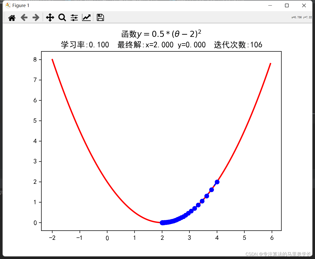
6. Results Plotting
X = np.arange(-2, 6, 0.05)
Y = np.array(list(map(lambda t: f1(t), X)))

plt.figure(facecolor='w')
plt.plot(X, Y, 'r-', linewidth=2)
plt.plot(GD_X, GD_Y, 'bo--', linewidth=2)
plt.title(f'function $y=0.5 * (θ - 2)^2$ \\
Learning rate: {<!-- -->alpha:.3f} Final solution: x={<!-- -->x:.3f} y={<!-- -->f_current:.3f} Number of iterations:{<!-- -->iter_num}')
plt. show()
You can try different starting points by yourself, and the impact of different learning rates on the results.

3 multivariate function gradient descent sample code
When the number of variables is 2, gradient descent can be shown using 3D plots. When the variable book exceeds 2, the loss function becomes a hyperplane and it is difficult to display, so here we take the binary function as an example.
- Defines the function to be simulated this time.
# binary function definition
def f2(x, y):
    return (x - 2) ** 2 + 2* (y + 1) ** 2
# Partial derivative
def hx2(x, y):
    return 2*(x - 2)
def hy2(x, y):
    return 4*(y + 1)
Same as the unary function, we directly define the partial derivative of the function to reduce the code not related to this blog.
2. Initialize the parameters in gradient descent
GD_X1 = []
GD_X2 = []
GD_Y = []
x1 = 4
x2 = 4
alpha = 0.01
f_change = 1
f_current = f2(x1, x2)
GD_X1.append(x1)
GD_X2.append(x2)
GD_Y.append(f_current)
iter_num = 0
The parameters here are basically the same as those of the unary function, except that there is an additional listGD_X2 for storing additional dimensions.
3. Cycles of Gradient Descent Steps
while f_change > 1e-10 and iter_num < 1000:
    iter_num += 1
    prex1 = x1
    prex2 = x2
    x1 = x1 - alpha * hx2(prex1, prex2)
    x2 = x2 - alpha * hy2(prex1, prex2)

    tmp = f2(x1, x2)
    f_change = np.abs(f_current - tmp)
    f_current = tmp
    GD_X1.append(x1)
    GD_X2.append(x2)
    GD_Y.append(f_current)

print(u"The final result is: (%.3f, %.3f, %.3f)" % (x1, x2, f_current))
print(u"Number of iterations:%d" % iter_num)
The logic here is basically the same as for unary functions. For each x, the corresponding partial derivative is multiplied by the learning rate to obtain a new value of x. The same is true for multivariate functions with more than two variables.
The result of the operation is:

- drawing
X1 = np.arange(-5, 5, 0.2)
X2 = np.arange(-5, 5, 0.2)
X1, X2 = np.meshgrid(X1, X2)
Y = np.array(list(map(lambda t: f2(t[0], t[1]), zip(X1.flatten(), X2.flatten()))))
Y.shape = X1.shape

fig = plt.figure(facecolor='w')
ax = Axes3D(fig)
ax.plot_surface(X1, X2, Y, rstride=1, cstride=1, cmap=plt.cm.jet, alpha=0.8)
ax.plot(GD_X1, GD_X2, GD_Y, 'ko-')
ax.set_xlabel('x')
ax.set_ylabel('y')
ax.set_zlabel('z')
plt. show()
For 3D data, we used meshgrid to construct a plotting grid for plotting function graphs. After drawing the function image, draw the image of each step of gradient descent. When drawing a line chart, ko- represents black, dots, and dotted lines.
(It is recommended to set the 3D image to be displayed separately, so that it is convenient to drag the viewing angle to view)

In fact, there are many types of gradient descent, such as stochastic gradient descent, batch gradient descent, and small batch gradient descent. These will be explained in the next blog.