1. ElasticSearch document score_score calculationUnderlying principle
Lucene (or Elasticsearch) uses a Boolean model to find matching documents and a formula called a practical scoring function to calculate relevance. This formula draws on term frequency/inverse document frequency and vector space model, and also adds some modern new features, such as coordination factor and field length normalization. (field length normalization), and word or query statement weight improvement.
Boolean model
Boolean Model Just use AND, OR and NOT (AND, OR and NOT) in queries ) to find matching documents, the following query:
full AND text AND search AND (elasticsearch OR lucene)
Will include all words full, text and search, as well as elasticsearch or lucene documents as a result set.
The process is simple and fast, and it excludes all potentially unmatched documents.
Term frequency/inverse document frequency (TF/IDF)
When a set of documents is matched, these documents need to be sorted according to relevance. Not all documents contain all words, and some words are more important than others. A document’s relevance score depends in part on the weight of each query term in the document.
Word frequency
How often does the word appear in the document? The higher the frequency, the higher the weight. A field with 5 mentions of the same word is more relevant than one with just 1 mention. Word frequency is calculated as follows:
tf(t in d) = √frequency
The word frequency ( tf ) of word t in document d is the square root of the number of times the word appears in the document.
If you don’t care about the frequency of a word appearing in a certain field, but only care about whether it has appeared before, you can disable word frequency statistics in the field mapping:
PUT /my_index
{
  "mappings": {
    "doc": {
      "properties": {
        "text": {
          "type": "string",
          "index_options": "docs"
        }
      }
    }
  }
}
Setting the parameter index_options to docs disables word frequency statistics and word frequency positions. This mapped field does not count word occurrences and is not available for phrase or approximate queries. not_analyzed string fields that require precise queries will use this setting by default.
Reverse document frequency
How often does the word appear in all documents in the collection? The higher the frequency, the lower the weight. Common words like and or the contribute little to relevance because they appear in most documents, and some uncommon words like elastic or hippopotamus can help us quickly narrow down the scope to find the documents of interest. The formula for calculating reverse document frequency is as follows:
idf(t) = 1 + log ( numDocs / (docFreq + 1))
The inverse document frequency ( idf ) of the word t is the logarithm of the number of documents in the index divided by the number of documents containing the word.
Field length normalized value
What is the length of the field? The shorter the field, the higher the weight of the field. If a word appears in a field like title, it will be more relevant than if it appears in a field like body. The normalized value formula of field length is as follows:
norm(d) = 1 / √numTerms
The field length normalization value ( norm ) is the reciprocal of the square root of the number of words in the field.
Normalization of field lengths is important for full-text searches, and many other fields do not require normalization. Each string field takes up approximately 1 byte of space for each document in the index, regardless of whether the document contains this field. For not_analyzed string fields, normalization of values is disabled by default, and for analyzed fields, normalization can also be disabled by modifying the field mapping:
PUT /my_index
{
  "mappings": {
    "doc": {
      "properties": {
        "text": {
          "type": "string",
          "norms": { "enabled": false }
        }
      }
    }
  }
}
This field does not take field length normalization into account; long and short fields are scored at the same length.
For some application scenarios such as logging, normalized values are not very useful. All you need to care about is whether the field contains a special error code or a specific browser unique identifier. The length of the field has no effect on the result, and disabling normalization can save a lot of memory space.
Use in combination
The following three factors-term frequency, inverse document frequency, and field-length norm-are calculated and stored at index time. Finally, they are combined to calculate the weight of a single word in a specific document.
The document mentioned in the previous formula actually refers to a certain field in the document. Each field has its own inverted index, so the TF/IDF value of the field is the TF/IDF of the document. value.
When viewing a simple term query using explain (see explain ), you can see that the factors used to calculate the relevance score are those introduced in the previous chapter:
PUT /my_index/doc/1
{ "text" : "quick brown fox" }

GET /my_index/doc/_search?explain
{
  "query": {
    "term": {
      "text": "fox"
    }
  }
}
The (simplified) explanation of the above request is as follows:
weight(text:fox in 0) [PerFieldSimilarity]: 0.15342641
result of:
fieldWeight in 0 0.15342641
product of:
tf(freq=1.0), with freq of 1: 1.0
idf(docFreq=1, maxDocs=1): 0.30685282
fieldNorm(doc=0): 0.5
Word fox Inside the document the Lucene doc ID is 0 and the field is The final score in text. |
|
|---|---|
The word fox is in the text field of this document Appeared only once. |
|
fox The inverse document frequency indexed by the text field in all documents. |
|
| The field length normalized value of this field. |
Of course, queries often have more than one word, so a way to combine the weights of multiple words is needed – a vector space model.
Vector space model
Vector space model provides a way to compare multi-word queries. A single score represents how well the document matches the query. To do this, this model combines both the document and the query with < Em>Vectors are expressed in the form of:
A vector is actually a one-dimensional array containing multiple numbers, for example:
[1,2,5,22,3,8]
In the vector space model, each number in the vector space model represents the weight of a word, which is similar to the calculation method of term frequency/inverse document frequency.
Although TF/IDF is the default way for vector space models to calculate word weights, it is not the only way. Elasticsearch also has other models such as Okapi-BM25. TF/IDF is the default because it is a proven simple and efficient algorithm that provides high-quality search results.
Imagine that if you query “happy hippopotamus”, the common word happy has a lower weight, and the uncommon word hippopotamus has a higher weight. Assume that the weight of happy is 2. The weight of hippopotamus is 5. This two-dimensional vector – [2,5] – can be used to draw a straight line in the coordinate system. The starting point of the line is ( 0,0) The end point is (2,5), as shown in Figure 27, “Two-dimensional query vector representing “happy hippopotamus””.
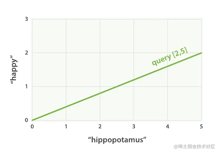
Figure 27. Two-dimensional query vector representing “happy hippopotamus”
Now, imagine we have three documents:
- I am happy in summer.
- After Christmas I’m ahippopotamus.
- Thehappy hippopotamus helped Harry.
You can create a vector containing the weight of each query term – happy and hippopotamus – for each document, and then place these vectors into the same coordinate system, such as Figure 28, ““happy hippopotamus” query and document vector”:
- Document 1:
(happy,____________)—[2,0] - Document 2:
( ___ ,hippopotamus)—[0,5] - Document 3:
(happy,hippopotamus)—[2,5]
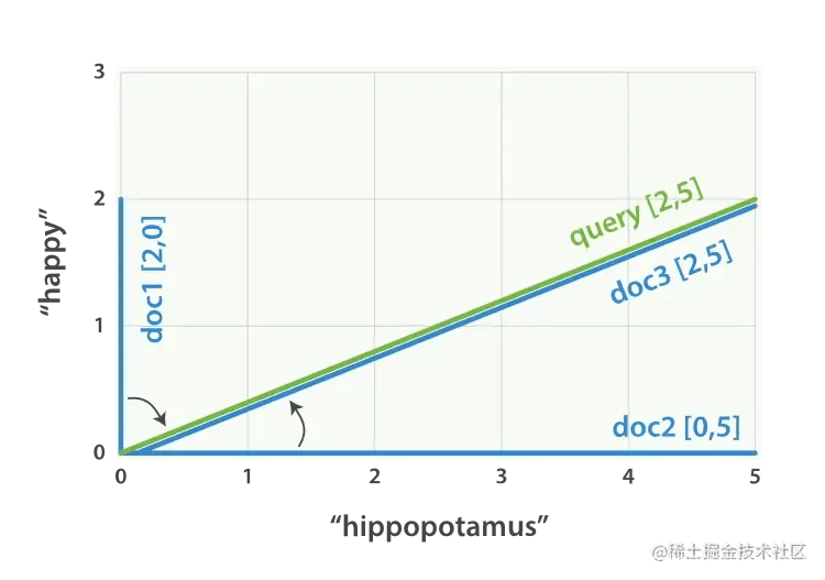
Figure 28. “happy hippopotamus” query and document vectors
Vectors can be compared. As long as the angle between the query vector and the document vector is measured, the correlation of each document can be obtained. The angle between document 1 and the query is the largest, so the correlation is low; the correlation between document 2 and the query is The angle is smaller, so it is more relevant; document 3 exactly matches the angle of the query, a perfect match.
Score calculation formula score(q,d) =
queryNorm(q) //Normalization factor · coord(q,d) //Coordination factor · ∑ (
tf(t in d) //Term frequency · idf(t)2 //Inverse document frequency · t.getBoost() //Weight · norm(t,d) //Field length normalized value) (t in q)
The following is a brief introduction to the three newly mentioned parameters in the formula:
queryNorm Query normalization factor: will be applied to each document, cannot be changed, and in short, can be ignored.
coord Coordination factor: It can provide rewards for documents with high query term inclusion. The more query terms appear in the document, the more likely it is to become a good matching result.
The coordination factor multiplies the score by the number of matching words in the document and then divides it by the number of all words in the query. If the coordination factor is used, the score becomes:
There is fox in the document → Rating: 1.5 * 1 / 3 = 0.5 There is quick fox in the document → Rating: 3.0 * 2 / 3 = 2.0 There is quick brown fox in the document → Rating: 4.5 * 3 / 3 = 4.5 The coordination factor enables the inclusion Documents with all three words are rated much higher than documents with only two words.
Boost weight: Setting the weight of keywords in the query can flexibly find more matching documents.
test preparation
PUT /demo
PUT /demo/_mapping { "properties":{ "content":{ "type":"text" } } }
GET demo
POST demo/_doc { "content": "Test statement 3, field lengths are different" } POST /demo/_search{" query":{"match":{"content":"test"}}}
{
  "took" : 792,
  "timed_out" : false,
  "_shards" : {
    "total" : 1,
    "successful" : 1,
    "skipped" : 0,
    "failed" : 0
  },
  "hits" : {
    "total" : {
      "value" : 3,
      "relation" : "eq"
    },
    "max_score" : 0.15120466,
    "hits" : [
      {
        "_index" : "demo",
        "_type" : "_doc",
        "_id" : "narolH0Byb0W9gti_JAl",
        "_score" : 0.15120466,
        "_source" : {
          "content" : "Test statement 1"
        }
      },
      {
        "_index" : "demo",
        "_type" : "_doc",
        "_id" : "nqrplH0Byb0W9gtiaZA_",
        "_score" : 0.15120466,
        "_source" : {
          "content" : "Test statement 2"
        }
      },
      {
        "_index" : "demo",
        "_type" : "_doc",
        "_id" : "n6rplH0Byb0W9gti2pCm",
        "_score" : 0.108230695,
        "_source" : {
          "content" : "Test statement 3, field lengths are different"
        }
      }
    ]
  }
}
As you can see, the scoring is as we expected. Documents 1 and 2 have the same score, while document 3 has a lower score because it is longer.
Continue to test the impact of weights on queries
POST /demo/_search?search_type=dfs_query_then_fetch
{
  "query": {
    "bool": {
      "should": [
        {
          "match": {
            "content": { "query": "1", "boost": 2 } }
        },
        {
          "match": {
            "content": "2" }
        }
      ]
    }
  }
}
result
{
  "took" : 109,
  "timed_out" : false,
  "_shards" : {
    "total" : 1,
    "successful" : 1,
    "skipped" : 0,
    "failed" : 0
  },
  "hits" : {
    "total" : {
      "value" : 2,
      "relation" : "eq"
    },
    "max_score" : 2.2212896,
    "hits" : [
      {
        "_index" : "demo",
        "_type" : "_doc",
        "_id" : "narolH0Byb0W9gti_JAl",
        "_score" : 2.2212896,
        "_source" : {
          "content" : "Test statement 1"
        }
      },
      {
        "_index" : "demo",
        "_type" : "_doc",
        "_id" : "nqrplH0Byb0W9gtiaZA_",
        "_score" : 1.1106448,
        "_source" : {
          "content" : "Test statement 2"
        }
      }
    ]
  }
}
As you can see, document 1 has a higher score than document 2 because the search keyword 1 is given a higher weight.
2. In-depth aggregation search technology
1. Introduction to the concepts of bucket and metric
Bucket is a data grouping during aggregate search. For example: the sales department has employees Zhang San and Li Si, and the development department has employees Wang Wu and Zhao Liu. Then the result of aggregation based on department grouping is two buckets. There are Zhang San and Li Si in the sales department bucket.
There are Wang Wu and Zhao Liu in the development department bucket.
A metric is a statistical analysis performed on a bucket’s data. As in the above case, there are 2 employees in the development department and 2 employees in the sales department. This is the metric.
Metric has various statistics, such as sum, maximum value, minimum value, average value, etc.
? Use a SQL syntax that is easy for everyone to understand, such as: select count() from table group by column. Then each group of data grouped by group by column is a bucket. The count() performed on each group is the metric.
2. Prepare case data
PUT /cars { "mappings": { "properties": { "price": { "type": "long" }, "color": { "type": "keyword" }, "brand": { "type": "keyword" }, "model": { "type": "keyword" }, "sold_date": { "type": "date" }, "remark" : { "type" : "text", "analyzer" : "ik_max_word" } } } }
POST /cars/_bulk { "index": {}} { "price" : 258000, "color" : "gold", "brand":"Volkswagen", "model" : "Volkswagen Magotan", "sold_date " : "2021-10-28", "remark" : "Volkswagen mid-range car" } { "index": {}} { "price" : 123000, "color" : "gold", "brand":"Volkswagen" , "model" : "Volkswagen Sagitar", "sold_date" : "2021-11-05", "remark" : "Volkswagen Sagitar" } { "index": {}} { "price" : 239800, "color" : "white", "brand":"Mark", "model" : "Mark 508", "sold_date" : "2021-05-18", "remark" : "Mark brand global launch models" } { "index" : {}} { "price" : 148800, "color" : "white", "brand":"LOGO", "model" : "LOGO 408", "sold_date" : "2021-07-02","remark " : "Relatively large compact car" } { "index": {}} { "price" : 1998000, "color" : "black", "brand": "Volkswagen", "model" : "Volkswagen Phaeton" , "sold_date" : "2021-08-19", "remark" : "Volkswagen's most painful car" } { "index": {}} { "price" : 218000, "color" : "red" , "brand": "Audi", "model" : "Audi A4", "sold_date" : "2021-11-05", "remark" : "petty bourgeoisie model" } { "index": {}} { "price " : 489000, "color" : "black", "brand": "Audi", "model" : "Audi A6", "sold_date" : "2022-01-01", "remark" : "For government use only?" } { "index": {}} { "price" : 1899000, "color" : "black", "brand": "Audi", "model" : "Audi A 8", "sold_date" : "2022-02 -12","remark" : "A very expensive big A6. . . " }
3. Aggregation operation case
3.1 Statistics of sales quantity according to color grouping
Only aggregate grouping is performed, and no complex aggregation statistics are performed. The most basic aggregation in ES is terms, which is equivalent to count in SQL.
In ES, grouped data is sorted by default, and doc_count data is used to perform descending order. You can use _key metadata to perform different sorting schemes based on grouped field data, or you can use _count metadata to perform different sorting schemes based on grouped statistical values.
GET /cars/_search
{
    "aggs":{
        "group_by_color":{
            "terms":{
                "field":"color",
                "order":{
                    "_count":"desc"
                }
            }
        }
    }
}
3.2 Statistics on the average price of vehicles of different colors
In this case, aggregation grouping is first performed based on color. Based on this grouping, aggregation statistics are performed on the data in the group. The aggregation statistics of the data in the group is metric. Sorting can also be performed because there are aggregate statistics in the group and the statistics are named avg_by_price, so the sorting logic can be performed based on the field name of the aggregate statistics.
GET /cars/_search
{
    "aggs":{
        "group_by_color":{
            "terms":{
                "field":"color",
                "order":{
                    "avg_by_price":"asc"
                }
            },
            "aggs":{
                "avg_by_price":{
                    "avg":{
                        "field":"price"
                    }
                }
            }
        }
    }
}
size can be set to 0, which means that the documents in ES will not be returned, but only the data after ES aggregation will be returned to improve the query speed. Of course, if you need these documents, you can also set them according to the actual situation.
GET /cars/_search
{
    "size":0,
    "aggs":{
        "group_by_color":{
            "terms":{
                "field":"color"
            },
            "aggs":{
                "group_by_brand":{
                    "terms":{
                        "field":"brand",
                        "order":{
                            "avg_by_price":"desc"
                        }
                    },
                    "aggs":{
                        "avg_by_price":{
                            "avg":{
                                "field":"price"
                            }
                        }
                    }
                }
            }
        }
    }
}
3.3 Statistics on the average price of vehicles in different colors and brands
First aggregate the groups according to color, and then aggregate the groups again according to brand within the group. This operation can be called drill-down analysis.
If there are many definitions of Aggs, the syntax format will be confusing. The syntax format of aggs has a relatively fixed structure and is simple to define: aggs can be nested and defined horizontally.
Nested definitions are called drill-down analysis. Horizontal definition is to tile multiple groups.
GET /index_name/type_name/_search
{
"aggs" : {
"Define group name (outermost)": {
"Group strategies such as: terms, avg, sum" : {
"field" : "Group according to which field",
\t\t\t\t"Other parameters" : ""
},
"aggs" : {
"Group name 1" : {},
"Group Name 2" : {}
}
}
}
}
GET /cars/_search
{
"aggs": {
"group_by_color": {
"terms": {
"field": "color",
"order": {
"avg_by_price_color": "asc"
}
},
"aggs": {
"avg_by_price_color": {
"avg": {
"field": "price"
}
},
"group_by_brand": {
"terms": {
"field": "brand",
"order": {
"avg_by_price_brand": "desc"
}
},
"aggs": {
"avg_by_price_brand": {
"avg": {
"field": "price"
}
}
}
}
}
}
}
}
3.4 Statistics on the maximum and minimum prices and total prices in different colors
GET /cars/_search
{
"aggs": {
"group_by_color": {
"terms": {
"field": "color"
},
"aggs": {
"max_price": {
"max": {
"field": "price"
}
},
"min_price": {
"min": {
"field": "price"
}
},
"sum_price": {
"sum": {
"field": "price"
}
}
}
}
}
}
In common business, aggregate analysis, the most commonly used types are statistical quantities, maximum, minimum, average, total, etc. It usually accounts for more than 60% of the aggregation business, and even accounts for more than 85% of small projects.
3.5 Statistics on the most expensive models among different brands of cars
After grouping, you may need to sort the data within the group and select the data with the highest ranking. Then you can use s to achieve it: the attribute size in top_top_hithits represents how many pieces of data are taken in the group (default is 10); sort represents what fields and rules are used in the group to sort (the default is to use _doc’s asc rule sorting); _source represents the results. Includes those fields in the document (default includes all fields).
GET cars/_search
{
"size": 0,
"aggs": {
"group_by_brand": {
"terms": {
"field": "brand"
},
"aggs": {
"top_car": {
"top_hits": {
"size": 1,
"sort": [{
"price": {
"order": "desc"
}
}],
"_source": {
"includes": ["model", "price"]
}
}
}
}
}
}
}
3.6 histogram interval statistics
Histogram is similar to terms, and also performs bucket grouping operations. It implements data interval grouping based on a field.
For example: taking 1 million as a range, count the sales volume and average price of vehicles in different ranges. Then when using histogram aggregation, field specifies the price field price. The interval range is 1 million – interval: 1000000. At this time, ES will divide the price price range into: [0, 1000000), [1000000, 2000000), [2000000, 3000000), etc., and so on. While dividing the interval, histogram will count the number of data similar to terms. You can use nested aggs to perform aggregation analysis on the data within the group after aggregation and grouping.
GET /cars/_search
{
"aggs": {
"histogram_by_price": {
"histogram": {
"field": "price",
"interval": 1000000
},
"aggs": {
"avg_by_price": {
"avg": {
"field": "price"
}
}
}
}
}
}
3.7 date_histogram interval grouping
date_histogram can perform interval aggregation grouping on fields of date type, such as monthly sales, annual sales, etc.
For example: on a monthly basis, count the sales quantity and total sales amount of cars in different months. At this time, you can use date_histogram to implement aggregation grouping, where field specifies the field used for aggregation grouping, interval specifies the interval (optional values are: year, quarter, month, week, day, hour, minute, second), format specifies the date For formatting, min_doc_count specifies the minimum document in each interval (if not specified, the default is 0, and when there is no document in the interval, the bucket group will also be displayed), extended_bounds specifies the start time and end time (if not specified, the default is used The range of the minimum value and maximum value of the date in the field is the start and end time).
After 7.X
GET /cars/_search
{
"aggs": {
"histogram_by_date": {
"date_histogram": {
"field": "sold_date",
"calendar_interval": "month",
"format": "yyyy-MM-dd",
"min_doc_count": 1,
"extended_bounds": {
"min": "2021-01-01",
"max": "2022-12-31"
}
},
"aggs": {
"sum_by_price": {
"sum": {
"field": "price"
}
}
}
}
}
}
3.8 _global bucket
When aggregating statistical data, sometimes it is necessary to compare partial data with overall data.
For example: Statistics of the average price of a certain brand of vehicles and the average price of all vehicles. global is used to define a global bucket. This bucket will ignore the query conditions and retrieve all documents for corresponding aggregation statistics.
GET /cars/_search
{
"size": 0,
"query": {
"match": {
"brand": "public"
}
},
"aggs": {
"volkswagen_of_avg_price": {
"avg": {
"field": "price"
}
},
"all_avg_price": {
"global": {},
"aggs": {
"all_of_price": {
"avg": {
"field": "price"
}
}
}
}
}
}
3.9 aggs + order
Sort aggregated statistics.
For example: count the car sales and total sales of each brand, and sort them in descending order of total sales.
GET /cars/_search
{
"aggs": {
"group_of_brand": {
"terms": {
"field": "brand",
"order": {
"sum_of_price": "desc"
}
},
"aggs": {
"sum_of_price": {
"sum": {
"field": "price"
}
}
}
}
}
}
If there are multiple levels of aggs, when performing drill-down aggregation, sorting can also be performed based on the innermost aggregation data.
For example: count the total sales of vehicles of each color in each brand, and sort them in descending order according to the total sales. This is just like group sorting in SQL. You can only sort data within a group, but not across groups.
GET /cars/_search
{
"aggs": {
"group_by_brand": {
"terms": {
"field": "brand"
},
"aggs": {
"group_by_color": {
"terms": {
"field": "color",
"order": {
"sum_of_price": "desc"
}
},
"aggs": {
"sum_of_price": {
"sum": {
"field": "price"
}
}
}
}
}
}
}
}
3.10 search + aggs
Aggregation is similar to the group by clause in SQL, and search is similar to the where clause in SQL. In ES, it is completely possible to integrate search and aggregations to perform relatively more complex search statistics.
For example: Statistics of sales and sales of a certain brand of vehicles each quarter.
GET /cars/_search
{
"query": {
"match": {
"brand": "public"
}
},
"aggs": {
"histogram_by_date": {
"date_histogram": {
"field": "sold_date",
"calendar_interval": "quarter",
"min_doc_count": 1
},
"aggs": {
"sum_by_price": {
"sum": {
"field": "price"
}
}
}
}
}
}
3.11 filter + aggs
In ES, filter can also be used in combination with aggs to implement relatively complex filtering and aggregation analysis.
For example: Statistics of the average price of vehicles between 100,000 and 500,000.
GET /cars/_search
{
"query": {
"constant_score": {
"filter": {
"range": {
"price": {
"gte": 100000,
"lte": 500000
}
}
}
}
},
"aggs": {
"avg_by_price": {
"avg": {
"field": "price"
}
}
}
}
3.12 Use filter in aggregation
filter can also be used in aggs syntax. The scope of filter determines the scope of its filtering.
For example: Statistics of the total sales of a certain brand of cars in the past year. Putting filter inside aggs means that this filter only performs filtering on the results obtained by query search. If filter is placed outside aggs, the filter will filter all data.
-
12M/M means 12 months.
-
1y/y means 1 year.
-
d means day
GET /cars/_search
{
"query": {
"match": {
"brand": "public"
}
},
"aggs": {
"count_last_year": {
"filter": {
"range": {
"sold_date": {
"gte": "now-12M"
}
}
},
"aggs": {
"sum_of_price_last_year": {
"sum": {
"field": "price"
}
}
}
}
}
}