Table of Contents
-
- 3.10.3 Histogram–3: Two-dimensional histogram
-
- Target
- introduction
- 2D histogram in OpenCV
- 2D histogram in Numpy
- Draw a 2D histogram
- 3.10.4 Histogram – 4: Histogram Backprojection
-
- Target
- theory
- Algorithms in Numpy
- Backprojection in OpenCV
- other resources
Translation and secondary proofreading: cvtutorials.com
Editor: Twenty Bottle Whale (Siby team member of Hejing Community)
3.10.3 Histogram–3: Two-dimensional histogram
Goal
In this chapter, we will learn how to find and plot a 2D histogram. It will be helpful for later chapters.
Introduction
In the first article, we calculated and plotted a 1D histogram. It is called one-dimensional because we only consider one feature, the grayscale gray value of the pixel. But in a 2D histogram, you have two features to consider. Typically, it is used to find color histograms, where two features are the hue and saturation values of each pixel.
There is already a python sample (samples/python/color_histogram.py) for finding a color histogram. We will try to understand how to create such a color histogram, which is useful for understanding further topics like histogram backprojection.
Two-dimensional histogram in OpenCV
It is very simple, using the same function cv.calcHist() to calculate. For the color histogram, we need to convert the image from BGR to HSV. (Remember, for 1D histograms we convert from BGR to grayscale). ) for a two-dimensional histogram, its parameters will be modified as follows.
- channels = [0,1] because we need to process both H and S planes.
- bins = [180,256] 180 for H plane and 256 for S plane.
- range = [0,180,0,256] Hue value between 0 and 180, saturation between 0 and 256.
Now look at the following code:
import numpy as np
import cv2 as cv
img = cv.imread('home.jpg')
hsv = cv.cvtColor(img,cv.COLOR_BGR2HSV)
hist = cv.calcHist([hsv], [0, 1], None, [180, 256], [0, 180, 0, 256])
2D histogram in Numpy
Numpy also provides a dedicated function: np.histogram2d(). (Remember, for a 1D histogram we use np.histogram() ).
import numpy as np
import cv2 as cv
from matplotlib import pyplot as plt
img = cv.imread('home.jpg')
hsv = cv.cvtColor(img,cv.COLOR_BGR2HSV)
hist, xbins, ybins = np.histogram2d(h.ravel(),s.ravel(),[180,256],[[0,180],[0,256]])
The first parameter is the H surface, the second is the S surface, the third is the number of bins, and the fourth is the range.
Now we can check how to plot this color histogram.
Draw a two-dimensional histogram
Method-1: Use cv.imshow()
The result we get is a 2D array of size 180×256. So we can display them with the cv.imshow() function as usual. This will be a grayscale image, and unless you know the hue values of the different colors, it won’t give a clue what colors are there.
Method-2: Using Matplotlib
We can use the matplotlib.pyplot.imshow() function to plot a 2D histogram with different color maps. This can give us a better understanding of different pixel densities. However, this also doesn’t let us know what color it is at first glance unless you know the hue values of the different colors. But I still like this approach. It’s simple and good.
Note: When using this function, keep in mind that for better results, the interpolation flag should be closest.
Take a look at the code:
import numpy as np
import cv2 as cv
from matplotlib import pyplot as plt
img = cv.imread('home.jpg')
hsv = cv.cvtColor(img,cv.COLOR_BGR2HSV)
hist = cv.calcHist( [hsv], [0, 1], None, [180, 256], [0, 180, 0, 256] )
plt.imshow(hist, interpolation = 'nearest')
plt. show()
Below is the input image and its color histogram map. The X-axis shows the S value and the Y-axis shows the hue.
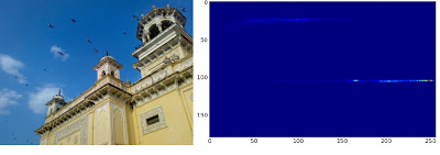
In the histogram, you can see some high values around H=100 and S=200. It corresponds to the blue of the sky. Likewise, another peak can be seen around H=25 and S=100. It corresponds to the yellow color of the palace. You can verify it with any image editing tool like GIMP.
Method 3: OpenCV sample style
In the OpenCV-Python2 sample (samples/python/color_histogram.py), there is a sample code for color histogram. If you run the code, you can see that the histogram shows the corresponding colors as well. Or simply, it outputs a color-coded histogram. It works pretty well (although you need to add a bunch of extra rows).
In that code, the author creates a colormap with HSV. Then convert it to BGR. The resulting histogram image is multiplied with this colormap. He also used some preprocessing steps to remove isolated small pixels, resulting in a nice histogram.
I leave it to the reader to run this code, analyze it, and think about it. Below is the output of this code for the same image above.
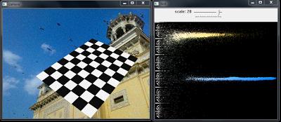
You can clearly see in the histogram which colors are present, blue is present, yellow is present, and some white due to the checkerboard is present.
3.10.4 Histogram – 4: Histogram backprojection
Goal
In this chapter, we will learn about histogram backprojection.
Theory
It was proposed by Michael J. Swain and Dana H. Ballard in their paper, indexing by color histogram.
Simply put, what exactly is it? It is used for image segmentation or finding objects of interest in an image. Simply put, it creates an image of the same size (but single-channel) as our input image, where each pixel corresponds to the probability that that pixel belongs to our object. In simpler terms, the output image will have more white in our object of interest compared to the rest. Well, that’s an intuitive explanation. Histogram backprojection is used with camshift algorithm etc.
How do we do it? We create a histogram of images containing the objects we are interested in (in our case, the ground, leaving players, and other things). For better results, objects should fill the image as much as possible. Color histograms are preferred over grayscale histograms because the color of an object defines the object more than its grayscale. Then, we “reverse ” this histogram on the test image where we need to find the object, that is, in other words, we calculate the probability of each pixel belonging to the ground and display it. The output after proper thresholding alone gives us information about the ground.
Algorithms in Numpy
1. First, we need to calculate the color histogram of the object we need to find (let’s call it “M”) and the image we want to search for (let’s call it “I”).
import numpy as np
import cv2 as cvfrom matplotlib import pyplot as plt
#roi is the object or region of object we need to find
roi = cv.imread('rose_red.png')
hsv = cv.cvtColor(roi,cv.COLOR_BGR2HSV)
#target is the image we search in
target = cv.imread('rose.png')
hsvt = cv.cvtColor(target,cv.COLOR_BGR2HSV)
# Find the histograms using calcHist. Can be done with np.histogram2d also
M = cv.calcHist([hsv],[0, 1], None, [180, 256], [0, 180, 0, 256] )
I = cv.calcHist([hsvt],[0, 1], None, [180, 256], [0, 180, 0, 256] )
2. Find the ratio R=M/I. Then reverse R, that is, use R as a palette to create a new image, and each pixel is its corresponding target probability. That is, B(x,y) = R[h(x,y),s(x,y)] where h is the hue and s is the saturation of the pixel at (x,y). Then apply the condition B(x,y)=min[B(x,y),1].
h,s,v = cv.split(hsvt)
B = R[h.ravel(),s.ravel()]
B = np.minimum(B,1)
B = B. reshape(hsvt. shape[:2])
3. Now apply a disk convolution, B=D?B, where D is the kernel of the disk.
disc = cv.getStructuringElement(cv.MORPH_ELLIPSE,(5,5))
cv. filter2D(B,-1, disc, B)
B = np.uint8(B)
cv.normalize(B,B,0,255,cv.NORM_MINMAX)
4. Now, the position of the maximum gray level gives us the position of the object. If we are looking for a region in an image, thresholding with an appropriate value will give a good result.
ret,thresh = cv.threshold(B,50,255,0)
Backprojection in OpenCV
OpenCV provides a built-in function cv.calcBackproject(). Its parameters are almost the same as cv.calcHist() function. One of its parameters is the histogram, which is the histogram of the object we have to find. Also, the object’s histogram should be normalized before passing to the backproject function. It returns a probability image. We then convolve the image with a disc kernel and apply a threshold. Below is my code and output.
import numpy as np
import cv2 as cv
roi = cv.imread('rose_red.png')
hsv = cv.cvtColor(roi,cv.COLOR_BGR2HSV)
target = cv.imread('rose.png')
hsvt = cv.cvtColor(target,cv.COLOR_BGR2HSV)
# calculating object histogram
roihist = cv.calcHist([hsv],[0, 1], None, [180, 256], [0, 180, 0, 256] )
# normalize histogram and apply backprojection
cv.normalize(roihist,roihist,0,255,cv.NORM_MINMAX)
dst = cv.calcBackProject([hsvt],[0,1],roihist,[0,180,0,256],1)
# Now convolute with circular disc
disc = cv.getStructuringElement(cv.MORPH_ELLIPSE,(5,5))
cv. filter2D(dst,-1, disc, dst)
# threshold and binary AND
ret,thresh = cv.threshold(dst,50,255,0)
thresh = cv. merge((thresh,thresh,thresh))
res = cv. bitwise_and(target,thresh)
res = np.vstack((target,thresh,res))
cv.imwrite('res.jpg',res)
Below is an example of what I’m dealing with. I take the area inside the blue rectangle as a sample object, and I want to extract the whole ground.

Additional resources
- “Indexing via color histograms”, Swain, Michael J. , Third international conference on computer vision, 1990.